Numpy Dot Function

Numpy Dot Function

NumPy is a powerful library for numerical computing in Python, and one of its most versatile and frequently used functions is the dot function. The numpy.dot() function is a fundamental tool for performing matrix multiplication and dot product operations on arrays. In this comprehensive guide, we’ll explore the various aspects of the numpy.dot() function, its applications, and provide numerous examples to illustrate its usage.

1. Introduction to numpy.dot()

The numpy.dot() function is used to compute the dot product of two arrays. It can be applied to 1-dimensional vectors, 2-dimensional matrices, and even higher-dimensional arrays. The behavior of the dot function depends on the dimensions of the input arrays.

Let’s start with a simple example to demonstrate the basic usage of numpy.dot():

import numpy as np

# Create two 1-dimensional arrays
a = np.array([1, 2, 3])
b = np.array([4, 5, 6])

# Compute the dot product
result = np.dot(a, b)

print("Arrays:")
print("a =", a)
print("b =", b)
print("Dot product of a and b:", result)
print("This example is from numpyarray.com")

Output:

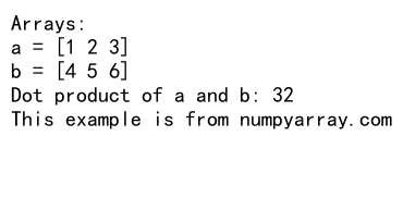
In this example, we create two 1-dimensional arrays a and b, and then use np.dot() to compute their dot product. The dot product of two vectors is the sum of the products of their corresponding elements.

2. Dot Product of Vectors

When applied to two 1-dimensional arrays (vectors), numpy.dot() computes the scalar dot product. This is equivalent to multiplying corresponding elements and summing the results.

Let’s look at a more detailed example:

import numpy as np

# Create two vectors
v1 = np.array([2, 3, -1])
v2 = np.array([4, -2, 1])

# Compute the dot product
dot_product = np.dot(v1, v2)

print("Vectors:")
print("v1 =", v1)
print("v2 =", v2)
print("Dot product of v1 and v2:", dot_product)
print("Step-by-step calculation:")
print("(2 * 4) + (3 * -2) + (-1 * 1) =", dot_product)
print("This example is from numpyarray.com")

Output:

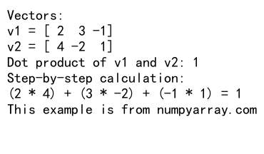
This example demonstrates how the dot product is calculated for two 3-dimensional vectors. The result is a scalar value obtained by multiplying corresponding elements and summing them up.

3. Matrix Multiplication

When numpy.dot() is applied to 2-dimensional arrays (matrices), it performs matrix multiplication. This is one of the most common use cases for the dot function in scientific computing and linear algebra applications.

Here’s an example of matrix multiplication using numpy.dot():

import numpy as np

# Create two matrices
A = np.array([[1, 2], [3, 4]])
B = np.array([[5, 6], [7, 8]])

# Perform matrix multiplication
C = np.dot(A, B)

print("Matrices:")
print("A =")
print(A)
print("B =")
print(B)
print("Result of A dot B:")
print(C)
print("This example is from numpyarray.com")

Output:

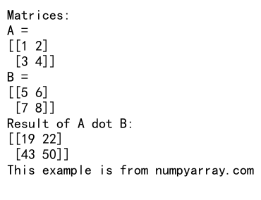
In this example, we multiply two 2×2 matrices. The resulting matrix C is also a 2×2 matrix. Each element in C is computed by taking the dot product of a row from A with a column from B.

4. Matrix-Vector Multiplication

The numpy.dot() function can also be used to multiply a matrix by a vector. This operation is common in many linear algebra applications, such as solving systems of linear equations.

Let’s see an example:

import numpy as np

# Create a matrix and a vector
M = np.array([[1, 2, 3], [4, 5, 6]])
v = np.array([7, 8, 9])

# Perform matrix-vector multiplication
result = np.dot(M, v)

print("Matrix M:")
print(M)
print("Vector v:", v)
print("Result of M dot v:", result)
print("This example is from numpyarray.com")

Output:

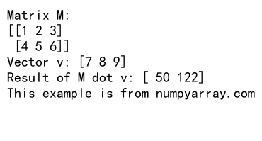
In this case, the result is a vector with the same number of rows as the matrix M. Each element of the result is the dot product of a row from M with the vector v.

5. Higher-Dimensional Array Operations

The numpy.dot() function can handle arrays with more than two dimensions. The behavior depends on the shapes of the input arrays and follows specific rules for contraction over the last axis of the first array and the second-to-last axis of the second array.

Here’s an example with 3-dimensional arrays:

import numpy as np

# Create two 3-dimensional arrays
A = np.array([[[1, 2], [3, 4]], [[5, 6], [7, 8]]])
B = np.array([[[9, 10], [11, 12]], [[13, 14], [15, 16]]])

# Perform dot product
C = np.dot(A, B)

print("Array A shape:", A.shape)
print("Array B shape:", B.shape)
print("Result C shape:", C.shape)
print("Result C:")
print(C)
print("This example is from numpyarray.com")

Output:

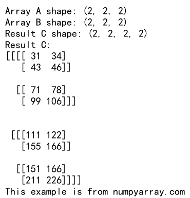
In this example, we’re working with 3-dimensional arrays. The dot product is computed along the last axis of A and the second-to-last axis of B. The result C is also a 3-dimensional array.

6. Dot Product with Scalar Multiplication

The numpy.dot() function can also handle scalar multiplication when one of the inputs is a scalar value. In this case, it behaves similarly to element-wise multiplication.

Let’s see an example:

import numpy as np

# Create an array and a scalar
arr = np.array([1, 2, 3, 4, 5])
scalar = 2

# Perform dot product with scalar
result = np.dot(arr, scalar)

print("Array:", arr)
print("Scalar:", scalar)
print("Result of arr dot scalar:", result)
print("This is equivalent to:", arr * scalar)
print("This example is from numpyarray.com")

Output:

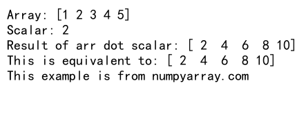
In this case, the dot product with a scalar is equivalent to multiplying each element of the array by the scalar value.

7. Dot Product vs. Element-wise Multiplication

It’s important to distinguish between the dot product (np.dot()) and element-wise multiplication (using the * operator). While they may produce the same result for 1-dimensional arrays, they behave differently for higher-dimensional arrays.

Let’s compare the two:

import numpy as np

# Create two arrays
a = np.array([1, 2, 3])
b = np.array([4, 5, 6])

# Dot product
dot_result = np.dot(a, b)

# Element-wise multiplication
element_wise_result = a * b

print("Array a:", a)
print("Array b:", b)
print("Dot product result:", dot_result)
print("Element-wise multiplication result:", element_wise_result)
print("This example is from numpyarray.com")

Output:

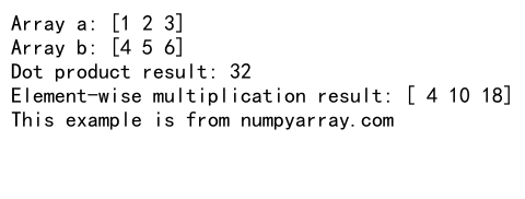
In this example, we can see that for 1-dimensional arrays, the dot product produces a scalar, while element-wise multiplication produces an array of the same shape as the input arrays.

8. Using numpy.dot() for Polynomial Evaluation

An interesting application of the numpy.dot() function is in evaluating polynomials. We can represent a polynomial as an array of coefficients and use dot product to efficiently compute its value for a given input.

Here’s an example:

import numpy as np

# Define polynomial coefficients (ax^2 + bx + c)
coefficients = np.array([2, -3, 1])  # 2x^2 - 3x + 1

# Define x values
x = np.array([0, 1, 2, 3, 4])

# Create array of powers of x
x_powers = np.array([x**0, x**1, x**2])

# Evaluate polynomial using dot product
y = np.dot(coefficients, x_powers)

print("Polynomial coefficients:", coefficients)
print("x values:", x)
print("Polynomial values:", y)
print("This example is from numpyarray.com")

Output:

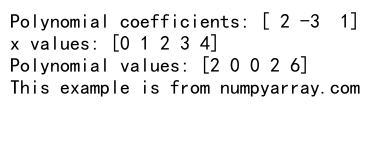
In this example, we evaluate the polynomial 2x^2 – 3x + 1 for multiple x values using a single dot product operation.

9. Solving Systems of Linear Equations

The numpy.dot() function is crucial in solving systems of linear equations. When combined with numpy.linalg.inv() for matrix inversion, we can implement the solution to Ax = b, where A is a matrix, and x and b are vectors.

Here’s an example:

import numpy as np

# Define the coefficient matrix A and the constant vector b
A = np.array([[2, 1], [1, 3]])
b = np.array([4, 5])

# Solve the system Ax = b
x = np.dot(np.linalg.inv(A), b)

print("Coefficient matrix A:")
print(A)
print("Constant vector b:", b)
print("Solution x:", x)
print("Verification (Ax):", np.dot(A, x))
print("This example is from numpyarray.com")

Output:

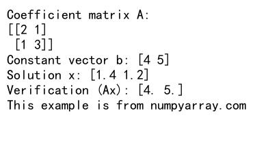
This example demonstrates how to solve a system of two linear equations using matrix operations and the dot product.

10. Implementing Neural Network Forward Pass

The dot product is fundamental in implementing neural networks. We can use numpy.dot() to perform the forward pass of a simple neural network layer.

Here’s a basic example:

import numpy as np

# Define input, weights, and bias
input_data = np.array([1, 2, 3])
weights = np.array([[0.1, 0.2, 0.3],
                    [0.4, 0.5, 0.6],
                    [0.7, 0.8, 0.9]])
bias = np.array([0.1, 0.2, 0.3])

# Perform forward pass
layer_output = np.dot(weights, input_data) + bias

# Apply activation function (e.g., ReLU)
activated_output = np.maximum(0, layer_output)

print("Input data:", input_data)
print("Weights:")
print(weights)
print("Bias:", bias)
print("Layer output before activation:", layer_output)
print("Activated output:", activated_output)
print("This example is from numpyarray.com")

Output:

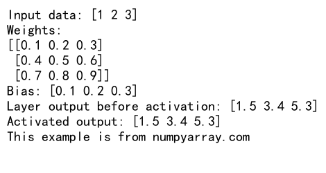
This example shows how to use numpy.dot() to compute the output of a neural network layer, followed by an activation function.

11. Computing Correlation Coefficient

The dot product can be used to compute the correlation coefficient between two variables. This is useful in statistical analysis and data science applications.

Here’s an example of how to compute the Pearson correlation coefficient:

import numpy as np

# Create two variables
x = np.array([1, 2, 3, 4, 5])
y = np.array([2, 4, 5, 4, 5])

# Compute means
x_mean = np.mean(x)
y_mean = np.mean(y)

# Center the variables
x_centered = x - x_mean
y_centered = y - y_mean

# Compute correlation coefficient
numerator = np.dot(x_centered, y_centered)
denominator = np.sqrt(np.dot(x_centered, x_centered) * np.dot(y_centered, y_centered))
correlation = numerator / denominator

print("Variable x:", x)
print("Variable y:", y)
print("Correlation coefficient:", correlation)
print("This example is from numpyarray.com")

Output:

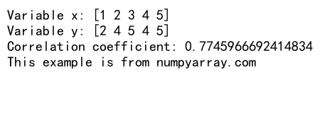
This example demonstrates how to use the dot product to compute the correlation coefficient between two variables.

12. Implementing Principal Component Analysis (PCA)

Principal Component Analysis is a dimensionality reduction technique that relies heavily on matrix operations, including the dot product. Here’s a simplified example of how to implement PCA using numpy.dot():

import numpy as np

# Create a sample dataset
X = np.array([[1, 2, 3], [4, 5, 6], [7, 8, 9], [10, 11, 12]])

# Center the data
X_centered = X - np.mean(X, axis=0)

# Compute the covariance matrix
cov_matrix = np.dot(X_centered.T, X_centered) / (X.shape[0] - 1)

# Compute eigenvectors and eigenvalues
eigenvalues, eigenvectors = np.linalg.eig(cov_matrix)

# Sort eigenvectors by decreasing eigenvalues
sorted_indices = np.argsort(eigenvalues)[::-1]
sorted_eigenvectors = eigenvectors[:, sorted_indices]

# Project the data onto the principal components
n_components = 2
principal_components = sorted_eigenvectors[:, :n_components]
projected_data = np.dot(X_centered, principal_components)

print("Original data shape:", X.shape)
print("Projected data shape:", projected_data.shape)
print("Principal components:")
print(principal_components)
print("This example is from numpyarray.com")

Output:

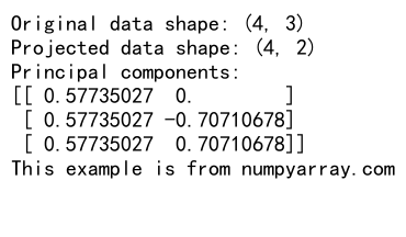
This example shows how to use numpy.dot() in various steps of the PCA process, including computing the covariance matrix and projecting the data onto the principal components.

13. Implementing Markov Chains

Markov chains are stochastic models used to describe a sequence of possible events. The transition between states in a Markov chain can be represented using a transition matrix, and the dot product is used to compute the probabilities of future states.

Here’s an example:

import numpy as np

# Define the transition matrix
P = np.array([[0.7, 0.2, 0.1],
              [0.3, 0.5, 0.2],
              [0.2, 0.3, 0.5]])

# Define initial state probabilities
initial_state = np.array([1, 0, 0])

# Compute probabilities after 1, 2, and 3 steps
step1 = np.dot(initial_state, P)
step2 = np.dot(step1, P)
step3 = np.dot(step2, P)

print("Transition matrix:")
print(P)
print("Initial state:", initial_state)
print("Probabilities after 1 step:", step1)
print("Probabilities after 2 steps:", step2)
print("Probabilities after 3 steps:", step3)
print("This example is from numpyarray.com")

Output:

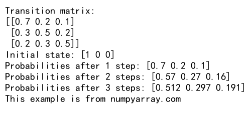
This example demonstrates how to use numpy.dot() to compute the state probabilities in a Markov chain after multiple steps.

14. Image Convolution

Convolution is a fundamental operation in image processing and computer vision. The numpy.dot() function can be used to implement a simple convolution operation.

Here’s an example of how to perform convolution on a small image:

import numpy as np

# Define a small image (3x3)
image = np.array([[1, 2, 3],
                  [4, 5, 6],
                  [7, 8, 9]])

# Define a kernel (2x2)
kernel = np.array([[1, 0],
                   [0, 1]])

# Pad the image
padded_image = np.pad(image, ((0, 1), (0, 1)), mode='constant')

# Perform convolution
result = np.zeros((3, 3))
for i in range(3):
    for j in range(3):
        result[i, j] = np.dot(padded_image[i:i+2, j:j+2].flatten(), kernel.flatten())

print("Original image:")
print(image)
print("Kernel:")
print(kernel)
print("Convolution result:")
print(result)
print("This example is from numpyarray.com")

Output:

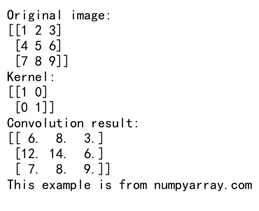
This example shows how to use numpy.dot() to implement a simple 2D convolution operation on an image.

15. Implementing Gradient Descent

Gradient descent is an optimization algorithm commonly used in machine learning. The dot product is used in computing the gradients and updating the parameters.

Here’s a simple example of implementing gradient descent for linear regression:

import numpy as np

# Generate some sample data
np.random.seed(42)
X = np.random.rand(100, 1)
y = 2 * X + 1 + np.random.randn(100, 1) * 0.1

# Initialize parameters
theta = np.random.randn(2, 1)

# Set hyperparameters
learning_rate = 0.1
num_iterations = 1000

# Gradient descent
for _ in range(num_iterations):
    # Compute predictions
    X_with_bias = np.hstack((np.ones((X.shape[0], 1)), X))
    y_pred = np.dot(X_with_bias, theta)

    # Compute gradients
    gradients = 2/X.shape[0] * np.dot(X_with_bias.T, (y_pred - y))

    # Update parameters
    theta -= learning_rate * gradients

print("Final parameters:")
print(theta)
print("This example is from numpyarray.com")

Output:

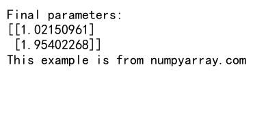
This example demonstrates how to use numpy.dot() in implementing gradient descent for linear regression, both for computing predictions and gradients.

16. Computing Cosine Similarity

Cosine similarity is a measure of similarity between two non-zero vectors. It’s widely used in text analysis and recommendation systems. The dot product is a key component in calculating cosine similarity.

Here’s an example:

import numpy as np

# Define two vectors
a = np.array([1, 2, 3])
b = np.array([4, 5, 6])

# Compute cosine similarity
dot_product = np.dot(a, b)
norm_a = np.linalg.norm(a)
norm_b = np.linalg.norm(b)
cosine_similarity = dot_product / (norm_a * norm_b)

print("Vector a:", a)
print("Vector b:", b)
print("Cosine similarity:", cosine_similarity)
print("This example is from numpyarray.com")

Output:

This example shows how to use numpy.dot() to compute the cosine similarity between two vectors.

17. Implementing PageRank Algorithm

The PageRank algorithm, used by Google to rank web pages, relies heavily on matrix operations including the dot product. Here’s a simplified implementation:

import numpy as np

# Define the adjacency matrix
A = np.array([[0, 1, 1, 0],
              [0, 0, 1, 0],
              [1, 0, 0, 1],
              [0, 0, 1, 0]])

# Number of pages
n = A.shape[0]

# Create the transition probability matrix
P = A / A.sum(axis=1, keepdims=True)

# Define damping factor
d = 0.85

# Initialize PageRank vector
pr = np.ones(n) / n

# Iterate to compute PageRank
for _ in range(100):
    pr_next = (1 - d) / n + d * np.dot(P.T, pr)
    if np.allclose(pr, pr_next):
        break
    pr = pr_next

print("PageRank values:")
print(pr)
print("This example is from numpyarray.com")

Output:

This example demonstrates how to use numpy.dot() in implementing the PageRank algorithm, which is essentially a series of matrix-vector multiplications.

18. Implementing Collaborative Filtering

Collaborative filtering is a technique used in recommendation systems. The dot product is used to compute the similarity between users or items. Here’s a simple example of user-based collaborative filtering:

import numpy as np

# User-item rating matrix
ratings = np.array([
    [4, 3, 0, 5, 0],
    [5, 0, 4, 0, 2],
    [3, 1, 2, 4, 1],
    [0, 0, 0, 2, 0],
    [1, 0, 3, 0, 0]
])

# Compute user similarity matrix
user_similarity = np.dot(ratings, ratings.T)

# Normalize similarity scores
user_similarity = user_similarity / np.linalg.norm(ratings, axis=1)[:, np.newaxis]
user_similarity = user_similarity / np.linalg.norm(ratings, axis=1)

# Make predictions for a user
user_id = 0
item_id = 2  # Item that the user hasn't rated

# Find similar users who have rated the item
mask = (ratings[:, item_id] > 0) & (np.arange(len(ratings)) != user_id)
similar_users = user_similarity[user_id, mask]
similar_ratings = ratings[mask, item_id]

# Compute weighted average of ratings
prediction = np.dot(similar_users, similar_ratings) / np.sum(similar_users)

print("User-item rating matrix:")
print(ratings)
print(f"Predicted rating for user {user_id} on item {item_id}: {prediction}")
print("This example is from numpyarray.com")

Output:

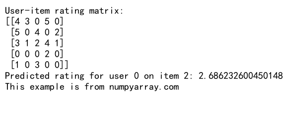
This example shows how to use numpy.dot() to compute user similarities and make predictions in a collaborative filtering system.

19. Implementing Discrete Fourier Transform

The Discrete Fourier Transform (DFT) is a fundamental tool in signal processing. The numpy.dot() function can be used to implement a simple version of the DFT.

Here’s an example:

import numpy as np

def dft(x):
    N = len(x)
    n = np.arange(N)
    k = n.reshape((N, 1))
    M = np.exp(-2j * np.pi * k * n / N)
    return np.dot(M, x)

# Generate a simple signal
t = np.linspace(0, 1, 100)
signal = np.sin(2 * np.pi * 10 * t) + 0.5 * np.sin(2 * np.pi * 20 * t)

# Compute DFT
spectrum = dft(signal)

print("Signal shape:", signal.shape)
print("Spectrum shape:", spectrum.shape)
print("First 10 values of the spectrum magnitude:")
print(np.abs(spectrum[:10]))
print("This example is from numpyarray.com")

Output:

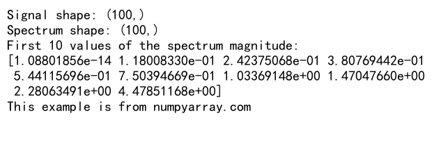
This example demonstrates how to use numpy.dot() to implement the Discrete Fourier Transform.

20. Implementing Support Vector Machine (SVM)

Support Vector Machines are powerful classifiers used in machine learning. The dot product is used in the kernel trick, which allows SVMs to operate in high-dimensional feature spaces. Here’s a simple example of a linear SVM using the dot product:

import numpy as np

class LinearSVM:
    def __init__(self, learning_rate=0.01, lambda_param=0.01, n_iters=1000):
        self.lr = learning_rate
        self.lambda_param = lambda_param
        self.n_iters = n_iters
        self.w = None
        self.b = None

    def fit(self, X, y):
        n_samples, n_features = X.shape
        self.w = np.zeros(n_features)
        self.b = 0

        for _ in range(self.n_iters):
            for idx, x_i in enumerate(X):
                condition = y[idx] * (np.dot(x_i, self.w) - self.b) >= 1
                if condition:
                    self.w -= self.lr * (2 * self.lambda_param * self.w)
                else:
                    self.w -= self.lr * (2 * self.lambda_param * self.w - np.dot(x_i, y[idx]))
                    self.b -= self.lr * y[idx]

    def predict(self, X):
        return np.sign(np.dot(X, self.w) - self.b)

# Generate some sample data
X = np.array([[1, 2], [2, 3], [3, 4], [4, 5], [5, 6], [-1, -2], [-2, -3], [-3, -4], [-4, -5], [-5, -6]])
y = np.array([1, 1, 1, 1, 1, -1, -1, -1, -1, -1])

# Train the SVM
svm = LinearSVM()
svm.fit(X, y)

# Make predictions
predictions = svm.predict(X)

print("Predictions:", predictions)
print("This example is from numpyarray.com")

Output:

This example shows how to use numpy.dot() in implementing a simple linear Support Vector Machine, both in the training process and for making predictions.

In conclusion, the numpy.dot() function is a versatile and powerful tool in numerical computing and data science. Its applications range from basic vector operations to complex machine learning algorithms. By understanding and mastering the use of numpy.dot(), you can efficiently implement a wide variety of mathematical and computational tasks in your data science projects.

Remember that while numpy.dot() is highly optimized for performance, for very large-scale operations or specific use cases, you might want to consider using specialized libraries like BLAS (Basic Linear Algebra Subprograms) or GPU-accelerated libraries like CuPy for even better performance.

As you continue to work with NumPy and explore more advanced topics in data science and machine learning, you’ll find that the dot product and the numpy.dot() function are fundamental building blocks that appear in many different contexts. Mastering their use will greatly enhance your ability to implement efficient and effective algorithms in your data science projects.