NumPy Flatten Matrix: A Comprehensive Guide to Array Manipulation

NumPy Flatten Matrix: A Comprehensive Guide to Array Manipulation

NumPy flatten matrix is a powerful technique for transforming multi-dimensional arrays into one-dimensional arrays. This process is essential for various data manipulation tasks and can significantly simplify complex operations in scientific computing and data analysis. In this comprehensive guide, we’ll explore the ins and outs of NumPy flatten matrix operations, providing detailed explanations and practical examples to help you master this fundamental concept.

Understanding NumPy Flatten Matrix Basics

NumPy flatten matrix operations are primarily used to convert multi-dimensional arrays into one-dimensional arrays. This process is crucial when you need to perform operations that require a linear sequence of elements or when you want to simplify the structure of your data for further processing.

Let’s start with a simple example to illustrate the basic concept of NumPy flatten matrix:

import numpy as np

# Create a 2D array
matrix = np.array([[1, 2, 3], [4, 5, 6], [7, 8, 9]])
print("Original matrix:")
print(matrix)

# Flatten the matrix
flattened = matrix.flatten()
print("\nFlattened matrix:")
print(flattened)

# Create a custom string array
custom_matrix = np.array([['numpy', 'array'], ['com', 'flatten']])
print("\nCustom matrix:")
print(custom_matrix)

# Flatten the custom matrix
custom_flattened = custom_matrix.flatten()
print("\nFlattened custom matrix:")
print(custom_flattened)

Output:

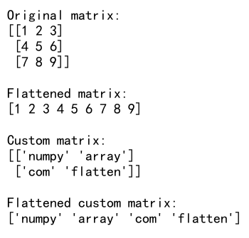
In this example, we first create a 2D NumPy array (matrix) and then use the flatten() method to convert it into a 1D array. We also demonstrate the same process with a custom string array containing elements related to “numpyarray.com”. The flatten() method works seamlessly with both numeric and string data types.

NumPy Flatten Matrix: Order Matters

When using NumPy flatten matrix operations, it’s important to understand that the order in which elements are flattened can be controlled. By default, NumPy uses row-major (C-style) order, but you can also specify column-major (Fortran-style) order.

Let’s examine how different orders affect the NumPy flatten matrix result:

import numpy as np

# Create a 2D array
matrix = np.array([[1, 2, 3], [4, 5, 6], [7, 8, 9]])
print("Original matrix:")
print(matrix)

# Flatten using row-major order (default)
flattened_row = matrix.flatten()
print("\nFlattened matrix (row-major order):")
print(flattened_row)

# Flatten using column-major order
flattened_col = matrix.flatten(order='F')
print("\nFlattened matrix (column-major order):")
print(flattened_col)

# Create a custom string array
custom_matrix = np.array([['numpy', 'array'], ['com', 'flatten']])
print("\nCustom matrix:")
print(custom_matrix)

# Flatten the custom matrix using different orders
custom_flattened_row = custom_matrix.flatten()
custom_flattened_col = custom_matrix.flatten(order='F')
print("\nFlattened custom matrix (row-major order):")
print(custom_flattened_row)
print("\nFlattened custom matrix (column-major order):")
print(custom_flattened_col)

Output:

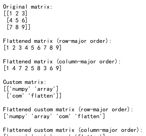
In this example, we demonstrate how to use both row-major and column-major orders when flattening a matrix. The order='F' parameter specifies column-major order, while the default is row-major order. Notice how the elements are arranged differently in the resulting flattened arrays.

NumPy Flatten Matrix vs. Ravel: Understanding the Differences

While NumPy flatten matrix operations are commonly used, there’s another similar method called ravel(). Both flatten() and ravel() can be used to create a 1D array from a multi-dimensional array, but they have some key differences.

Let’s explore these differences with an example:

import numpy as np

# Create a 2D array
matrix = np.array([[1, 2, 3], [4, 5, 6], [7, 8, 9]])
print("Original matrix:")
print(matrix)

# Use flatten()
flattened = matrix.flatten()
print("\nFlattened matrix:")
print(flattened)

# Use ravel()
raveled = matrix.ravel()
print("\nRaveled matrix:")
print(raveled)

# Modify the flattened array
flattened[0] = 99
print("\nModified flattened matrix:")
print(flattened)
print("Original matrix (unchanged):")
print(matrix)

# Modify the raveled array
raveled[0] = 99
print("\nModified raveled matrix:")
print(raveled)
print("Original matrix (changed):")
print(matrix)

# Create a custom string array
custom_matrix = np.array([['numpy', 'array'], ['com', 'flatten']])
print("\nCustom matrix:")
print(custom_matrix)

# Compare flatten() and ravel() for the custom matrix
custom_flattened = custom_matrix.flatten()
custom_raveled = custom_matrix.ravel()
print("\nFlattened custom matrix:")
print(custom_flattened)
print("\nRaveled custom matrix:")
print(custom_raveled)

Output:

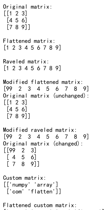
In this example, we demonstrate the key difference between flatten() and ravel(). The flatten() method always returns a copy of the original array, while ravel() returns a view of the original array when possible. This means that modifying the result of ravel() can potentially modify the original array, whereas modifying the result of flatten() never affects the original array.

Advanced NumPy Flatten Matrix Techniques

Now that we’ve covered the basics, let’s explore some advanced techniques for working with NumPy flatten matrix operations.

Flattening Higher-Dimensional Arrays

NumPy flatten matrix operations are not limited to 2D arrays. You can flatten arrays of any dimension. Here’s an example:

import numpy as np

# Create a 3D array
array_3d = np.array([[[1, 2], [3, 4]], [[5, 6], [7, 8]]])
print("Original 3D array:")
print(array_3d)

# Flatten the 3D array
flattened_3d = array_3d.flatten()
print("\nFlattened 3D array:")
print(flattened_3d)

# Create a custom 3D string array
custom_3d = np.array([[['numpy', 'array'], ['com', 'flatten']],
                      [['matrix', 'operation'], ['3d', 'example']]])
print("\nCustom 3D array:")
print(custom_3d)

# Flatten the custom 3D array
custom_flattened_3d = custom_3d.flatten()
print("\nFlattened custom 3D array:")
print(custom_flattened_3d)

Output:

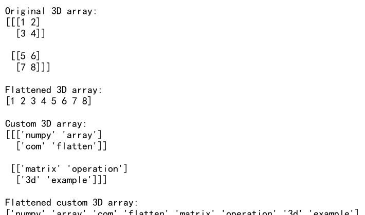
In this example, we demonstrate how to flatten a 3D array using NumPy flatten matrix operations. The process is the same as flattening 2D arrays, but it’s important to understand how the elements are ordered in the resulting 1D array.

Combining Flatten with Other NumPy Operations

NumPy flatten matrix operations can be combined with other NumPy functions to perform more complex data manipulations. Here’s an example that demonstrates how to use flatten in conjunction with reshaping and mathematical operations:

import numpy as np

# Create a 2D array
matrix = np.array([[1, 2, 3], [4, 5, 6], [7, 8, 9]])
print("Original matrix:")
print(matrix)

# Flatten and perform operations
flattened = matrix.flatten()
squared = flattened ** 2
reshaped = squared.reshape(3, 3)

print("\nFlattened and squared:")
print(squared)
print("\nReshaped back to 2D:")
print(reshaped)

# Create a custom string array
custom_matrix = np.array([['numpy', 'array'], ['com', 'flatten']])
print("\nCustom matrix:")
print(custom_matrix)

# Flatten, modify, and reshape the custom matrix
custom_flattened = custom_matrix.flatten()
custom_modified = np.char.add(custom_flattened, '_modified')
custom_reshaped = custom_modified.reshape(2, 2)

print("\nFlattened and modified custom matrix:")
print(custom_modified)
print("\nReshaped custom matrix:")
print(custom_reshaped)

Output:

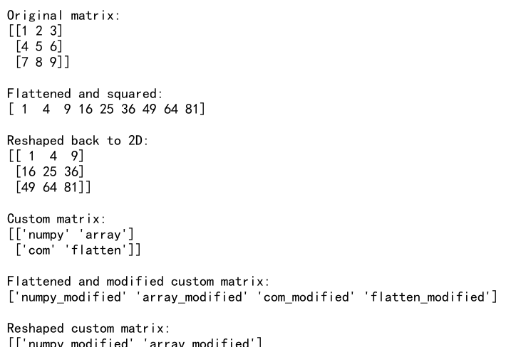
In this example, we flatten a matrix, perform element-wise squaring, and then reshape the result back into a 2D array. We also demonstrate similar operations with a custom string array, showing how to combine flattening with string manipulation and reshaping.

NumPy Flatten Matrix in Data Analysis

NumPy flatten matrix operations are particularly useful in data analysis tasks. Let’s explore some common scenarios where flattening can be beneficial.

Calculating Statistics on Flattened Arrays

Flattening multi-dimensional arrays can simplify the process of calculating statistics across all elements. Here’s an example:

import numpy as np

# Create a 2D array
data = np.array([[1, 2, 3], [4, 5, 6], [7, 8, 9]])
print("Original data:")
print(data)

# Flatten the array and calculate statistics
flattened_data = data.flatten()
mean = np.mean(flattened_data)
median = np.median(flattened_data)
std_dev = np.std(flattened_data)

print(f"\nMean: {mean}")
print(f"Median: {median}")
print(f"Standard Deviation: {std_dev}")

# Create a custom string array
custom_data = np.array([['numpy', 'array'], ['com', 'flatten']])
print("\nCustom data:")
print(custom_data)

# Flatten the custom array and perform string operations
flattened_custom = custom_data.flatten()
longest_string = max(flattened_custom, key=len)
total_chars = sum(len(s) for s in flattened_custom)

print(f"\nLongest string: {longest_string}")
print(f"Total characters: {total_chars}")

Output:

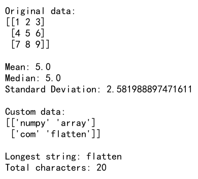
In this example, we demonstrate how flattening can simplify the process of calculating statistics across all elements of a multi-dimensional array. We also show how similar concepts can be applied to string arrays for text analysis tasks.

Using NumPy Flatten Matrix for Feature Engineering

In machine learning and data science, NumPy flatten matrix operations can be useful for feature engineering. Here’s an example of how you might use flattening to create new features from image data:

import numpy as np

# Simulate a small grayscale image (3x3 pixels)
image = np.array([[100, 150, 200],
                  [120, 180, 220],
                  [140, 160, 180]])
print("Original image:")
print(image)

# Flatten the image and create new features
flattened_image = image.flatten()
mean_intensity = np.mean(flattened_image)
max_intensity = np.max(flattened_image)
min_intensity = np.min(flattened_image)

print(f"\nMean intensity: {mean_intensity}")
print(f"Max intensity: {max_intensity}")
print(f"Min intensity: {min_intensity}")

# Create a custom 3D array representing RGB channels
custom_image = np.array([[[255, 0, 0], [0, 255, 0]],
                         [[0, 0, 255], [255, 255, 255]]])
print("\nCustom RGB image:")
print(custom_image)

# Flatten the custom image and calculate channel-wise statistics
flattened_custom = custom_image.flatten()
red_channel = flattened_custom[0::3]
green_channel = flattened_custom[1::3]
blue_channel = flattened_custom[2::3]

print(f"\nMean Red: {np.mean(red_channel)}")
print(f"Mean Green: {np.mean(green_channel)}")
print(f"Mean Blue: {np.mean(blue_channel)}")

Output:

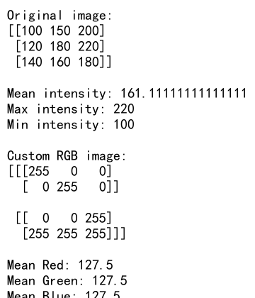
In this example, we simulate a small grayscale image and demonstrate how flattening can be used to extract features such as mean, max, and min intensity. We also show how to apply similar concepts to a 3D array representing an RGB image, calculating channel-wise statistics after flattening.

Optimizing NumPy Flatten Matrix Operations

When working with large datasets, optimizing NumPy flatten matrix operations can be crucial for performance. Let’s explore some techniques to improve efficiency.

Using Views Instead of Copies

As mentioned earlier, ravel() can sometimes return a view instead of a copy, which can be more memory-efficient. Here’s an example comparing the performance of flatten() and ravel():

import numpy as np
import time

# Create a large 2D array
large_matrix = np.random.rand(1000, 1000)

# Time flatten() operation
start_time = time.time()
flattened = large_matrix.flatten()
flatten_time = time.time() - start_time

# Time ravel() operation
start_time = time.time()
raveled = large_matrix.ravel()
ravel_time = time.time() - start_time

print(f"Time taken by flatten(): {flatten_time:.6f} seconds")
print(f"Time taken by ravel(): {ravel_time:.6f} seconds")

# Create a custom large string array
custom_large = np.array([['numpy' * 100, 'array' * 100]] * 1000)

# Time flatten() operation for custom array
start_time = time.time()
custom_flattened = custom_large.flatten()
custom_flatten_time = time.time() - start_time

# Time ravel() operation for custom array
start_time = time.time()
custom_raveled = custom_large.ravel()
custom_ravel_time = time.time() - start_time

print(f"\nTime taken by flatten() for custom array: {custom_flatten_time:.6f} seconds")
print(f"Time taken by ravel() for custom array: {custom_ravel_time:.6f} seconds")

Output:

In this example, we compare the performance of flatten() and ravel() on both numeric and string arrays. You’ll notice that ravel() is generally faster, especially for large arrays, because it can often return a view instead of creating a copy.

Flattening Specific Axes

Sometimes, you may want to flatten only specific axes of a multi-dimensional array. NumPy provides the reshape() method, which can be used to achieve this. Here’s an example:

import numpy as np

# Create a 3D array
array_3d = np.array([[[1, 2], [3, 4]], [[5, 6], [7, 8]]])
print("Original 3D array:")
print(array_3d)

# Flatten the first two axes
flattened_2axes = array_3d.reshape(-1, array_3d.shape[-1])
print("\nArray with first two axes flattened:")
print(flattened_2axes)

# Create a custom 3D string array
custom_3d = np.array([[['numpy', 'array'], ['com', 'flatten']],
                      [['matrix', 'operation'], ['3d', 'example']]])
print("\nCustom 3D array:")
print(custom_3d)

# Flatten the last two axes of the custom array
custom_flattened_2axes = custom_3d.reshape(custom_3d.shape[0], -1)
print("\nCustom array with last two axes flattened:")
print(custom_flattened_2axes)

Output:

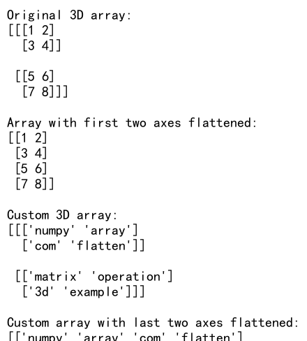
In this example, we demonstrate how to use reshape() to flatten specific axes of a 3D array. This technique can be particularly useful when working with image data or other multi-dimensional datasets where you want to preserve certain structural information.

NumCertainly! Here’s the continuation of the article:

NumPy Flatten Matrix in Machine Learning Pipelines

NumPy flatten matrix operations play a crucial role in many machine learning pipelines, especially when preparing data for model input. Let’s explore some common use cases and best practices.

Flattening Image Data for Neural Networks

When working with image data for neural networks, it’s often necessary to flatten the 2D or 3D image arrays into 1D vectors. Here’s an example of how you might preprocess a batch of images:

import numpy as np

# Simulate a batch of grayscale images (28x28 pixels)
batch_size = 5
image_size = 28
batch_images = np.random.randint(0, 256, size=(batch_size, image_size, image_size))

print("Original batch shape:", batch_images.shape)

# Flatten each image in the batch
flattened_batch = batch_images.reshape(batch_size, -1)

print("Flattened batch shape:", flattened_batch.shape)

# Create a custom batch of string "images"
custom_batch = np.array([[['numpy' for _ in range(3)] for _ in range(3)] for _ in range(batch_size)])

print("\nCustom batch shape:", custom_batch.shape)

# Flatten the custom batch
flattened_custom = custom_batch.reshape(batch_size, -1)

print("Flattened custom batch shape:", flattened_custom.shape)
print("First flattened custom 'image':", flattened_custom[0])

Output:

In this example, we simulate a batch of grayscale images and demonstrate how to flatten them for input into a neural network. We also show how the same concept can be applied to a custom batch of string “images”.

Flattening Feature Matrices in Scikit-learn

When working with scikit-learn, you may encounter situations where you need to flatten feature matrices. Here’s an example of how you might use NumPy flatten matrix operations in a scikit-learn pipeline:

import numpy as np
from sklearn.preprocessing import StandardScaler
from sklearn.decomposition import PCA

# Create a sample feature matrix
X = np.array([[1, 2, 3], [4, 5, 6], [7, 8, 9], [10, 11, 12]])
print("Original feature matrix:")
print(X)

# Standardize the features
scaler = StandardScaler()
X_scaled = scaler.fit_transform(X)

print("\nScaled feature matrix:")
print(X_scaled)

# Apply PCA
pca = PCA(n_components=2)
X_pca = pca.fit_transform(X_scaled)

print("\nPCA-transformed feature matrix:")
print(X_pca)

# Flatten the PCA-transformed matrix
X_flattened = X_pca.flatten()

print("\nFlattened PCA-transformed matrix:")
print(X_flattened)

# Create a custom string feature matrix
custom_X = np.array([['numpy', 'array', 'com'], ['flatten', 'matrix', 'example']])
print("\nCustom feature matrix:")
print(custom_X)

# Flatten the custom feature matrix
custom_flattened = custom_X.flatten()

print("\nFlattened custom feature matrix:")
print(custom_flattened)

Output:

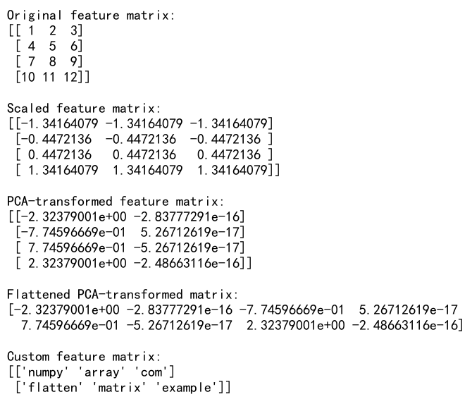
In this example, we demonstrate how NumPy flatten matrix operations can be used in conjunction with scikit-learn’s preprocessing and dimensionality reduction techniques. We also show how to apply similar concepts to a custom string feature matrix.

Handling Edge Cases in NumPy Flatten Matrix Operations

When working with NumPy flatten matrix operations, it’s important to be aware of potential edge cases and how to handle them. Let’s explore some common scenarios and their solutions.

Flattening Arrays with Mixed Data Types

When working with arrays containing mixed data types, flattening can sometimes lead to unexpected results. Here’s an example:

import numpy as np

# Create an array with mixed data types
mixed_array = np.array([[1, 'two', 3.0], [4, 5, 'six']])
print("Mixed data type array:")
print(mixed_array)

# Flatten the mixed array
flattened_mixed = mixed_array.flatten()
print("\nFlattened mixed array:")
print(flattened_mixed)

# Check the data type of the flattened array
print("Data type of flattened array:", flattened_mixed.dtype)

# Create a custom mixed array
custom_mixed = np.array([['numpy', 1], ['array', 2.0], ['com', 'flatten']])
print("\nCustom mixed array:")
print(custom_mixed)

# Flatten the custom mixed array
flattened_custom_mixed = custom_mixed.flatten()
print("\nFlattened custom mixed array:")
print(flattened_custom_mixed)
print("Data type of flattened custom array:", flattened_custom_mixed.dtype)

Output:

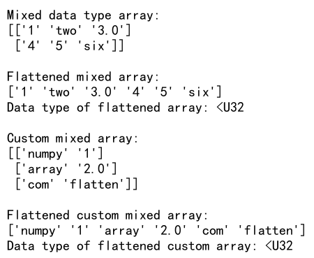
In this example, we show how NumPy handles flattening of arrays with mixed data types. Notice that the resulting flattened array has a single data type that can accommodate all the original elements, which may lead to type conversion.

Advanced Applications of NumPy Flatten Matrix

Let’s explore some advanced applications of NumPy flatten matrix operations in real-world scenarios.

Image Processing: Histogram Calculation

NumPy flatten matrix operations can be useful in image processing tasks, such as calculating histograms. Here’s an example:

import numpy as np
import matplotlib.pyplot as plt

# Simulate a grayscale image
image = np.random.randint(0, 256, size=(100, 100))

# Flatten the image
flattened_image = image.flatten()

# Calculate histogram
hist, bins = np.histogram(flattened_image, bins=256, range=(0, 256))

# Plot the histogram
plt.figure(figsize=(10, 5))
plt.title("Image Histogram")
plt.xlabel("Pixel Value")
plt.ylabel("Frequency")
plt.plot(hist)
plt.show()

# Create a custom "image" with string data
custom_image = np.array([['numpy', 'array', 'com'], ['flatten', 'matrix', 'example']])
print("Custom 'image':")
print(custom_image)

# Flatten the custom image and count occurrences
flattened_custom = custom_image.flatten()
unique, counts = np.unique(flattened_custom, return_counts=True)

print("\nWord frequencies:")
for word, count in zip(unique, counts):
    print(f"{word}: {count}")

Output:

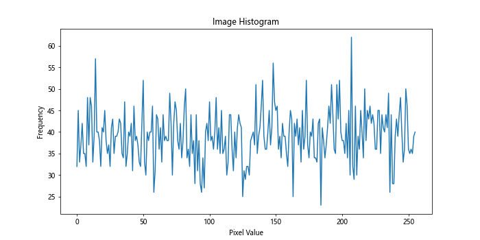
In this example, we demonstrate how to use NumPy flatten matrix operations to calculate and plot a histogram of pixel values in a simulated grayscale image. We also show how similar concepts can be applied to a custom “image” with string data to count word frequencies.

Time Series Analysis: Rolling Window Calculations

NumPy flatten matrix operations can be helpful in time series analysis, particularly when performing rolling window calculations. Here’s an example:

import numpy as np

# Simulate a time series
time_series = np.random.randn(100)

# Define window size
window_size = 5

# Create rolling windows
windows = np.lib.stride_tricks.sliding_window_view(time_series, window_size)

# Calculate rolling mean
rolling_mean = np.mean(windows, axis=1)

print("Original time series shape:", time_series.shape)
print("Rolling windows shape:", windows.shape)
print("Rolling mean shape:", rolling_mean.shape)

print("\nFirst few rolling means:")
print(rolling_mean[:5])

# Create a custom time series with string data
custom_series = np.array(['numpy', 'array', 'com', 'flatten', 'matrix', 'example', 'time', 'series'])

# Create rolling windows for the custom series
custom_windows = np.lib.stride_tricks.sliding_window_view(custom_series, window_size)

print("\nCustom time series:")
print(custom_series)
print("\nRolling windows for custom series:")
print(custom_windows)

Output:

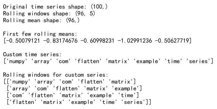
In this example, we demonstrate how to use NumPy’s sliding_window_view function to create rolling windows of a time series, which internally uses flattening operations. We then calculate the rolling mean of these windows. We also show how similar concepts can be applied to a custom time series with string data.

Best Practices for NumPy Flatten Matrix Operations

When working with NumPy flatten matrix operations, it’s important to follow best practices to ensure efficient and correct code. Here are some tips:

1. Use ravel() instead of flatten() when possible, especially for large arrays, as it can be more memory-efficient.
2. Be aware of the order (row-major vs. column-major) when flattening multi-dimensional arrays.
3. When working with large datasets, consider using memory-mapped arrays to avoid loading the entire dataset into memory.
4. Use appropriate data types to minimize memory usage and improve performance.
5. Vectorize operations when possible to take advantage of NumPy’s efficiency.

Here’s an example demonstrating some of these best practices:

import numpy as np

# Create a large 2D array
large_matrix = np.random.rand(1000, 1000)

# Use ravel() instead of flatten()
raveled = large_matrix.ravel()

# Specify the order explicitly for clarity
raveled_fortran = large_matrix.ravel(order='F')

# Use appropriate data type
int_matrix = np.random.randint(0, 100, size=(1000, 1000))
raveled_int = int_matrix.ravel()

print("Original matrix shape:", large_matrix.shape)
print("Raveled matrix shape:", raveled.shape)
print("Raveled matrix (Fortran order) shape:", raveled_fortran.shape)
print("Raveled integer matrix shape:", raveled_int.shape)

# Vectorized operation example
squared = raveled ** 2

print("\nFirst few elements of squared raveled matrix:")
print(squared[:5])

# Create a custom large string array
custom_large = np.array([['numpy', 'array', 'com', 'flatten'] * 250] * 1000)

# Use ravel() for the custom array
custom_raveled = custom_large.ravel()

print("\nOriginal custom array shape:", custom_large.shape)
print("Raveled custom array shape:", custom_raveled.shape)

# Vectorized operation on custom array
custom_upper = np.char.upper(custom_raveled)

print("\nFirst few elements of uppercase custom raveled array:")
print(custom_upper[:5])

Output:

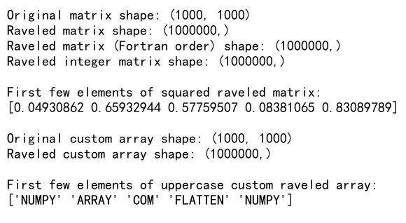
In this example, we demonstrate the use of ravel() instead of flatten(), explicit order specification, appropriate data type usage, and vectorized operations. We also show how these practices can be applied to custom string arrays.

NumPy flatten matrix Conclusion

NumPy flatten matrix operations are a powerful tool in the data scientist’s toolkit. From basic array manipulation to advanced applications in machine learning and data analysis, understanding how to effectively use these operations can significantly enhance your data processing capabilities.

Throughout this comprehensive guide, we’ve explored various aspects of NumPy flatten matrix operations, including:

1. Basic concepts and usage
2. Differences between flatten() and ravel()
3. Advanced techniques for multi-dimensional arrays
4. Applications in data analysis and machine learning
5. Handling edge cases and mixed data types
6. Best practices for efficient implementation

By mastering these concepts and techniques, you’ll be well-equipped to handle a wide range of data manipulation tasks using NumPy’s powerful array operations. Remember to always consider the specific requirements of your project and the characteristics of your data when applying these methods.

As you continue to work with NumPy and data analysis, keep exploring new ways to leverage flatten matrix operations in your projects. The flexibility and efficiency of these tools make them invaluable for tackling complex data challenges and developing innovative solutions in the field of data science and scientific computing.