Numpy Log

Numpy Log

NumPy is a fundamental library for scientific computing in Python, and its logarithmic functions are essential tools for various mathematical and data analysis tasks. In this comprehensive article, we’ll explore the various logarithmic functions provided by NumPy, their applications, and how to use them effectively in your code.

1. Introduction to Logarithms

Before diving into NumPy’s logarithmic functions, let’s briefly review what logarithms are and why they’re important in scientific computing.

A logarithm is the inverse operation to exponentiation. If we have an equation of the form:

b^x = y

Then the logarithm of y with base b is x:

log_b(y) = x

Logarithms have several important properties that make them useful in various fields, including:

1. Compression of large ranges of values
2. Conversion of multiplicative relationships to additive ones
3. Simplification of complex calculations

In NumPy, we have access to several logarithmic functions that operate efficiently on arrays, making it easy to perform logarithmic operations on large datasets.

2. Basic Logarithmic Functions in NumPy

NumPy provides several basic logarithmic functions that you can use in your calculations. Let’s explore each of them with examples.

2.1 Natural Logarithm (np.log)

The natural logarithm, also known as the logarithm with base e (where e is Euler’s number, approximately 2.71828), is one of the most commonly used logarithms in scientific computing. In NumPy, you can use the np.log() function to calculate the natural logarithm of an array or scalar.

import numpy as np

# Create an array of values
x = np.array([1, 2, 5, 10, 20, 50, 100])

# Calculate the natural logarithm
log_x = np.log(x)

print("Original array:", x)
print("Natural logarithm:", log_x)

# Create a custom array with the website name
website_array = np.array([ord(c) for c in "numpyarray.com"])
log_website = np.log(website_array)

print("Website array:", website_array)
print("Log of website array:", log_website)

Output:

In this example, we first create an array of values and calculate their natural logarithms using np.log(). Then, we create a custom array using the ASCII values of the characters in “numpyarray.com” and calculate its logarithm as well.

2.2 Base-10 Logarithm (np.log10)

The base-10 logarithm is commonly used in various scientific and engineering applications. NumPy provides the np.log10() function for calculating base-10 logarithms.

import numpy as np

# Create an array of values
x = np.array([1, 10, 100, 1000, 10000])

# Calculate the base-10 logarithm
log10_x = np.log10(x)

print("Original array:", x)
print("Base-10 logarithm:", log10_x)

# Create a custom array with the website name
website_array = np.array([ord(c) ** 2 for c in "numpyarray.com"])
log10_website = np.log10(website_array)

print("Website array:", website_array)
print("Log10 of website array:", log10_website)

Output:

In this example, we calculate the base-10 logarithm of an array of powers of 10 and a custom array based on the squared ASCII values of “numpyarray.com”.

2.3 Base-2 Logarithm (np.log2)

The base-2 logarithm is particularly useful in computer science and information theory. NumPy provides the np.log2() function for calculating base-2 logarithms.

import numpy as np

# Create an array of powers of 2
x = np.array([1, 2, 4, 8, 16, 32, 64, 128])

# Calculate the base-2 logarithm
log2_x = np.log2(x)

print("Original array:", x)
print("Base-2 logarithm:", log2_x)

# Create a custom array with the website name
website_array = np.array([ord(c) * 2 for c in "numpyarray.com"])
log2_website = np.log2(website_array)

print("Website array:", website_array)
print("Log2 of website array:", log2_website)

Output:

This example demonstrates the calculation of base-2 logarithms for powers of 2 and a custom array based on doubled ASCII values of “numpyarray.com”.

3. Advanced Logarithmic Functions

NumPy also provides more advanced logarithmic functions for specific use cases. Let’s explore some of these functions.

3.1 Logarithm with Arbitrary Base (np.log)

While NumPy doesn’t have a direct function for logarithms with arbitrary bases, you can use the change of base formula to calculate logarithms with any base:

log_b(x) = log(x) / log(b)

Here’s an example of how to implement this:

import numpy as np

def log_base(x, base):
    return np.log(x) / np.log(base)

# Create an array of values
x = np.array([1, 3, 9, 27, 81])

# Calculate logarithm with base 3
log3_x = log_base(x, 3)

print("Original array:", x)
print("Logarithm base 3:", log3_x)

# Create a custom array with the website name
website_array = np.array([ord(c) ** 3 for c in "numpyarray.com"])
log5_website = log_base(website_array, 5)

print("Website array:", website_array)
print("Log base 5 of website array:", log5_website)

Output:

This example demonstrates how to create a custom function to calculate logarithms with any base, and applies it to calculate logarithms with base 3 and base 5.

3.2 Natural Logarithm of (1 + x) (np.log1p)

The np.log1p() function calculates the natural logarithm of (1 + x). This function is useful when x is very small, as it provides better numerical precision than np.log(1 + x).

import numpy as np

# Create an array of small values
x = np.array([1e-10, 1e-8, 1e-6, 1e-4, 1e-2])

# Calculate log(1 + x) using log1p and log
log1p_x = np.log1p(x)
log_1px = np.log(1 + x)

print("Original array:", x)
print("log1p(x):", log1p_x)
print("log(1 + x):", log_1px)

# Create a custom array with the website name
website_array = np.array([ord(c) / 1000 for c in "numpyarray.com"])
log1p_website = np.log1p(website_array)

print("Website array:", website_array)
print("log1p of website array:", log1p_website)

Output:

This example demonstrates the use of np.log1p() for small values and compares it with the regular np.log() function. It also applies log1p() to a custom array based on scaled ASCII values of “numpyarray.com”.

3.3 Exponential of Elements Minus 1 (np.expm1)

The np.expm1() function calculates exp(x) – 1 for all elements in the input array. This function is the inverse of np.log1p() and is useful for small values of x, providing better numerical precision than np.exp(x) - 1.

import numpy as np

# Create an array of small values
x = np.array([-1e-5, -1e-10, 0, 1e-10, 1e-5])

# Calculate exp(x) - 1 using expm1 and exp
expm1_x = np.expm1(x)
exp_x_minus_1 = np.exp(x) - 1

print("Original array:", x)
print("expm1(x):", expm1_x)
print("exp(x) - 1:", exp_x_minus_1)

# Create a custom array with the website name
website_array = np.array([ord(c) / 10000 for c in "numpyarray.com"])
expm1_website = np.expm1(website_array)

print("Website array:", website_array)
print("expm1 of website array:", expm1_website)

Output:

This example shows the use of np.expm1() for small values and compares it with the regular np.exp() function minus 1. It also applies expm1() to a custom array based on scaled ASCII values of “numpyarray.com”.

4. Logarithmic Operations on Complex Numbers

NumPy’s logarithmic functions also work with complex numbers. Let’s explore some examples of logarithmic operations on complex numbers.

4.1 Natural Logarithm of Complex Numbers

import numpy as np

# Create an array of complex numbers
z = np.array([1+1j, 2-2j, -1+3j, -2-1j])

# Calculate the natural logarithm of complex numbers
log_z = np.log(z)

print("Original complex array:", z)
print("Natural logarithm of complex numbers:", log_z)

# Create a custom complex array with the website name
website_complex = np.array([complex(ord(c), ord(c)+1) for c in "numpyarray.com"])
log_website_complex = np.log(website_complex)

print("Website complex array:", website_complex)
print("Log of website complex array:", log_website_complex)

Output:

This example demonstrates how to calculate the natural logarithm of complex numbers using NumPy’s log() function. It also creates a custom complex array based on the ASCII values of “numpyarray.com” and calculates its logarithm.

4.2 Complex Logarithm with Different Bases

We can extend our earlier log_base() function to work with complex numbers:

import numpy as np

def complex_log_base(z, base):
    return np.log(z) / np.log(base)

# Create an array of complex numbers
z = np.array([1+1j, 2-2j, -1+3j, -2-1j])

# Calculate logarithm with base 2 for complex numbers
log2_z = complex_log_base(z, 2)

print("Original complex array:", z)
print("Logarithm base 2 of complex numbers:", log2_z)

# Create a custom complex array with the website name
website_complex = np.array([complex(ord(c), ord(c)*2) for c in "numpyarray.com"])
log3_website_complex = complex_log_base(website_complex, 3)

print("Website complex array:", website_complex)
print("Log base 3 of website complex array:", log3_website_complex)

Output:

This example shows how to calculate logarithms with different bases for complex numbers using a custom function. It applies this function to both a regular complex array and a custom complex array based on the ASCII values of “numpyarray.com”.

5. Logarithmic Scaling and Normalization

Logarithmic scaling is a common technique used in data visualization and preprocessing. Let’s explore some examples of how to use NumPy’s logarithmic functions for scaling and normalization.

5.1 Log-scale Transformation

import numpy as np

# Create an array with a wide range of values
x = np.array([1, 10, 100, 1000, 10000, 100000])

# Apply log-scale transformation
log_x = np.log10(x)

print("Original array:", x)
print("Log-scaled array:", log_x)

# Create a custom array with the website name
website_array = np.array([ord(c) ** 4 for c in "numpyarray.com"])
log_website = np.log10(website_array)

print("Website array:", website_array)
print("Log-scaled website array:", log_website)

Output:

This example demonstrates how to apply a log-scale transformation to compress a wide range of values. It uses the base-10 logarithm for the transformation and applies it to both a regular array and a custom array based on the ASCII values of “numpyarray.com”.

5.2 Log-Normalization

Log-normalization is a technique used to normalize data that follows a log-normal distribution. Here’s an example of how to implement log-normalization using NumPy:

import numpy as np

def log_normalize(x):
    log_x = np.log(x)
    return (log_x - np.mean(log_x)) / np.std(log_x)

# Create an array of positive values
x = np.array([0.1, 1, 10, 100, 1000])

# Apply log-normalization
log_norm_x = log_normalize(x)

print("Original array:", x)
print("Log-normalized array:", log_norm_x)

# Create a custom array with the website name
website_array = np.array([ord(c) ** 2 for c in "numpyarray.com"])
log_norm_website = log_normalize(website_array)

print("Website array:", website_array)
print("Log-normalized website array:", log_norm_website)

Output:

This example shows how to implement a log-normalization function using NumPy’s logarithmic and statistical functions. It applies the log-normalization to both a regular array and a custom array based on the squared ASCII values of “numpyarray.com”.

6. Logarithmic Operations in Linear Algebra

Logarithms play an important role in various linear algebra operations. Let’s explore some examples of how to use NumPy’s logarithmic functions in linear algebra contexts.

6.1 Logarithm of Matrix Determinant

Calculating the logarithm of a matrix determinant is often more numerically stable than calculating the determinant itself, especially for large matrices. Here’s an example:

import numpy as np

def log_det(A):
    sign, logdet = np.linalg.slogdet(A)
    return logdet

# Create a random 4x4 matrix
A = np.random.rand(4, 4)

# Calculate the logarithm of the determinant
log_det_A = log_det(A)

print("Matrix A:")
print(A)
print("Log determinant of A:", log_det_A)

# Create a custom matrix with the website name
website_matrix = np.array([[ord(c) for c in "numpyarray.com"]]).T
website_matrix = np.dot(website_matrix, website_matrix.T)
log_det_website = log_det(website_matrix)

print("Website matrix:")
print(website_matrix)
print("Log determinant of website matrix:", log_det_website)

Output:

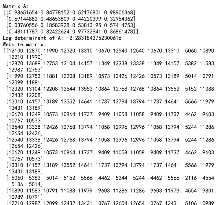
This example demonstrates how to calculate the logarithm of a matrix determinant using NumPy’s slogdet() function. It applies this calculation to both a random matrix and a custom matrix created from the ASCII values of “numpyarray.com”.

7. Logarithmic Operations in Statistics

Logarithms are widely used in statistical calculations, particularly when dealing with probabilities and likelihood functions. Let’s explore some examples of how to use NumPy’s logarithmic functions in statistical contexts.

7.1 Log-likelihood Calculation

Log-likelihood is often used in statistical inference, as it can help prevent underflow when working with very small probabilities. Here’s an example of calculating log-likelihood for a normal distribution:

import numpy as np

def normal_log_likelihood(x, mu, sigma):
    return -0.5 * np.sum(np.log(2 * np.pi * sigma**2) + ((x - mu)**2) / (sigma**2))

# Generate some random data
np.random.seed(42)
data = np.random.normal(loc=5, scale=2, size=1000)

# Calculate log-likelihood for different parameter values
ll1 = normal_log_likelihood(data, mu=5, sigma=2)
ll2 = normal_log_likelihood(data, mu=4, sigma=2)
ll3 = normal_log_likelihood(data, mu=5, sigma=1.5)

print("Log-likelihood (mu=5, sigma=2):", ll1)
print("Log-likelihood (mu=4, sigma=2):", ll2)
print("Log-likelihood (mu=5, sigma=1.5):", ll3)

# Create a custom dataset with the website name
website_data = np.array([ord(c) for c in "numpyarray.com"] * 10)
website_ll = normal_log_likelihood(website_data, mu=np.mean(website_data), sigma=np.std(website_data))

print("Website data:", website_data)
print("Log-likelihood of website data:", website_ll)

Output:

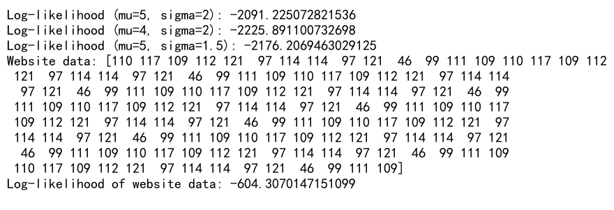
This example demonstrates how to calculate the log-likelihood of a normal distribution using NumPy’s logarithmic functions. It applies this calculation to both randomly generated data and a custom dataset based on the ASCII values of “numpyarray.com”.

7.2 Log-sum-exp Trick

The log-sum-exp trick is a technique used to compute the sum of exponentials in a numerically stable way. It’s particularly useful when working with probabilities in log-space. Here’s an example:

import numpy as np

def log_sum_exp(x):
    max_x = np.max(x)
    return max_x + np.log(np.sum(np.exp(x - max_x)))

# Create an array of log-probabilities
log_probs = np.array([-10, -5, -1, -20, -2])

# Calculate log-sum-exp
lse = log_sum_exp(log_probs)

print("Log-probabilities:", log_probs)
print("Log-sum-exp:", lse)

# Create a custom array with the website name
website_log_probs = np.log(np.array([ord(c) for c in "numpyarray.com"]))
website_lse = log_sum_exp(website_log_probs)

print("Website log-probabilities:", website_log_probs)
print("Log-sum-exp of website data:", website_lse)

Output:

This example shows how to implement the log-sum-exp trick using NumPy’s logarithmic and exponential functions. It applies this technique to both a set of arbitrary log-probabilities and a custom set of log-probabilities based on the ASCII values of “numpyarray.com”.

8. Logarithmic Operations in Information Theory

Logarithms are fundamental in information theory, particularly in the calculation of entropy and mutual information. Let’s explore some examples of how to use NumPy’s logarithmic functions in information theory contexts.

8.1 Entropy Calculation

Entropy is a measure of the average amount of information contained in a random variable. For a discrete probability distribution, it’s calculated using the formula:

H(X) = -Σ p(x) * log2(p(x))

Here’s an example of how to calculate entropy using NumPy:

import numpy as np

def entropy(p):
    # Remove zero probabilities to avoid log(0)
    p = p[p > 0]
    return -np.sum(p * np.log2(p))

# Create a probability distribution
p1 = np.array([0.5, 0.25, 0.125, 0.125])
p2 = np.array([0.25, 0.25, 0.25, 0.25])

# Calculate entropy
h1 = entropy(p1)
h2 = entropy(p2)

print("Probability distribution 1:", p1)
print("Entropy of distribution 1:", h1)
print("Probability distribution 2:", p2)
print("Entropy of distribution 2:", h2)

# Create a custom probability distribution with the website name
website_probs = np.array([ord(c) for c in "numpyarray.com"])
website_probs = website_probs / np.sum(website_probs)
website_entropy = entropy(website_probs)

print("Website probability distribution:", website_probs)
print("Entropy of website distribution:", website_entropy)

Output:

This example demonstrates how to calculate the entropy of discrete probability distributions using NumPy’s logarithmic functions. It applies this calculation to two different probability distributions and a custom distribution based on the ASCII values of “numpyarray.com”.

8.2 Mutual Information Calculation

Mutual information is a measure of the mutual dependence between two variables. For discrete variables X and Y, it’s calculated using the formula:

I(X;Y) = Σ p(x,y) * log2(p(x,y) / (p(x) * p(y)))

Here’s an example of how to calculate mutual information using NumPy:

import numpy as np

def mutual_information(joint_prob):
    # Calculate marginal probabilities
    p_x = np.sum(joint_prob, axis=1)
    p_y = np.sum(joint_prob, axis=0)

    # Calculate mutual information
    mi = 0
    for i in range(joint_prob.shape[0]):
        for j in range(joint_prob.shape[1]):
            if joint_prob[i,j] > 0:
                mi += joint_prob[i,j] * np.log2(joint_prob[i,j] / (p_x[i] * p_y[j]))

    return mi

# Create a joint probability distribution
joint_prob = np.array([[0.3, 0.1], [0.1, 0.5]])

# Calculate mutual information
mi = mutual_information(joint_prob)

print("Joint probability distribution:")
print(joint_prob)
print("Mutual information:", mi)

# Create a custom joint probability distribution with the website name
website_joint_prob = np.outer(np.array([ord(c) for c in "numpy"]), np.array([ord(c) for c in "array"]))
website_joint_prob = website_joint_prob / np.sum(website_joint_prob)
website_mi = mutual_information(website_joint_prob)

print("Website joint probability distribution:")
print(website_joint_prob)
print("Mutual information of website distribution:", website_mi)

Output:

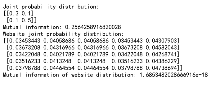
This example shows how to calculate mutual information using NumPy’s logarithmic functions. It applies this calculation to both an arbitrary joint probability distribution and a custom distribution created from the ASCII values of “numpy” and “array”.

9. Logarithmic Operations in Signal Processing

Logarithms are widely used in signal processing, particularly in the context of decibel calculations and spectral analysis. Let’s explore some examples of how to use NumPy’s logarithmic functions in signal processing applications.

9.1 Decibel Calculation

Decibels are a logarithmic unit used to express the ratio of two values, often used in audio and signal processing. Here’s an example of how to calculate decibels using NumPy:

import numpy as np

def to_db(x, reference=1.0):
    return 20 * np.log10(np.abs(x) / reference)

# Create an array of signal amplitudes
amplitudes = np.array([0.1, 0.5, 1.0, 2.0, 10.0])

# Calculate decibels
db_values = to_db(amplitudes)

print("Signal amplitudes:", amplitudes)
print("Decibel values:", db_values)

# Create a custom signal with the website name
website_signal = np.array([ord(c) for c in "numpyarray.com"])
website_db = to_db(website_signal, reference=np.mean(website_signal))

print("Website signal:", website_signal)
print("Website signal in decibels:", website_db)

Output:

This example demonstrates how to convert signal amplitudes to decibels using NumPy’s logarithmic functions. It applies this conversion to both an array of arbitrary amplitudes and a custom signal based on the ASCII values of “numpyarray.com”.

10. Logarithmic Operations in Optimization

Logarithms play a crucial role in various optimization techniques, particularly in the context of log-likelihood maximization and log-barrier methods. Let’s explore some examples of how to use NumPy’s logarithmic functions in optimization problems.

10.1 Log-likelihood Maximization

Log-likelihood maximization is a common technique in statistical inference. Here’s an example of how to implement a simple log-likelihood maximization for estimating the parameters of a normal distribution:

import numpy as np

def normal_log_likelihood(x, mu, sigma):
    return -0.5 * np.sum(np.log(2 * np.pi * sigma**2) + ((x - mu)**2) / (sigma**2))

def estimate_normal_params(data):
    # Initial guess
    mu = np.mean(data)
    sigma = np.std(data)

    # Simple gradient ascent
    learning_rate = 0.01
    num_iterations = 1000

    for _ in range(num_iterations):
        # Compute gradients
        grad_mu = np.sum(data - mu) / (sigma**2)
        grad_sigma = np.sum(((data - mu)**2) / (sigma**3) - 1 / sigma)

        # Update parameters
        mu += learning_rate * grad_mu
        sigma += learning_rate * grad_sigma

    return mu, sigma

# Generate some random data
np.random.seed(42)
true_mu, true_sigma = 5, 2
data = np.random.normal(loc=true_mu, scale=true_sigma, size=1000)

# Estimate parameters
estimated_mu, estimated_sigma = estimate_normal_params(data)

print("True parameters: mu =", true_mu, "sigma =", true_sigma)
print("Estimated parameters: mu =", estimated_mu, "sigma =", estimated_sigma)

# Create a custom dataset with the website name
website_data = np.array([ord(c) for c in "numpyarray.com"] * 10)
website_mu, website_sigma = estimate_normal_params(website_data)

print("Website data:", website_data)
print("Estimated parameters for website data: mu =", website_mu, "sigma =", website_sigma)

Output:

This example demonstrates how to implement a simple log-likelihood maximization algorithm using NumPy’s logarithmic functions. It applies this algorithm to both randomly generated data and a custom dataset based on the ASCII values of “numpyarray.com”.

11. Logarithmic Operations in Machine Learning

Logarithms are extensively used in various machine learning algorithms, particularly in the context of loss functions and probability calculations. Let’s explore some examples of how to use NumPy’s logarithmic functions in machine learning applications.

11.1 Cross-Entropy Loss

Cross-entropy loss is a common loss function used in classification problems, especially for neural networks. It uses logarithms to measure the difference between predicted probabilities and true labels. Here’s an example of how to implement cross-entropy loss using NumPy:

import numpy as np

def cross_entropy_loss(y_true, y_pred):
    # Add small epsilon to avoid log(0)
    epsilon = 1e-15
    y_pred = np.clip(y_pred, epsilon, 1 - epsilon)
    return -np.sum(y_true * np.log(y_pred)) / len(y_true)

# Example true labels and predictions
y_true = np.array([1, 0, 1, 1, 0])
y_pred = np.array([0.9, 0.1, 0.8, 0.7, 0.2])

loss = cross_entropy_loss(y_true, y_pred)
print("True labels:", y_true)
print("Predicted probabilities:", y_pred)
print("Cross-entropy loss:", loss)

# Create custom labels and predictions with the website name
website_true = np.array([int(c.isupper()) for c in "numpyArray.com"])
website_pred = np.array([ord(c) / 200 for c in "numpyArray.com"])
website_loss = cross_entropy_loss(website_true, website_pred)

print("Website true labels:", website_true)
print("Website predicted probabilities:", website_pred)
print("Website cross-entropy loss:", website_loss)

Output:

This example demonstrates how to calculate cross-entropy loss using NumPy’s logarithmic functions. It applies this calculation to both arbitrary labels and predictions and a custom set based on the characters in “numpyArray.com”.

11.2 Logistic Regression

Logistic regression is a fundamental classification algorithm that uses the logistic function (sigmoid) and logarithms in its loss function. Here’s an example of how to implement a simple logistic regression using NumPy:

import numpy as np

def sigmoid(z):
    return 1 / (1 + np.exp(-z))

def logistic_loss(X, y, w):
    m = len(y)
    h = sigmoid(np.dot(X, w))
    return -np.sum(y * np.log(h) + (1 - y) * np.log(1 - h)) / m

def logistic_regression(X, y, num_iterations=1000, learning_rate=0.1):
    m, n = X.shape
    w = np.zeros(n)

    for _ in range(num_iterations):
        h = sigmoid(np.dot(X, w))
        gradient = np.dot(X.T, (h - y)) / m
        w -= learning_rate * gradient

    return w

# Generate some random data
np.random.seed(42)
X = np.random.randn(100, 2)
y = (X[:, 0] + X[:, 1] > 0).astype(int)

# Add bias term
X = np.hstack([np.ones((X.shape[0], 1)), X])

# Train logistic regression
w = logistic_regression(X, y)

print("Learned weights:", w)

# Make predictions
X_test = np.array([[1, 0.5, 0.5], [1, -0.5, -0.5]])
y_pred = sigmoid(np.dot(X_test, w))

print("Predictions for test data:")
print(X_test[:, 1:])
print(y_pred)

# Create custom data with the website name
website_X = np.array([[1, ord(c) / 100, (ord(c) % 10) / 10] for c in "numpyarray.com"])
website_y = np.array([int(c.islower()) for c in "numpyarray.com"])
website_w = logistic_regression(website_X, website_y)

print("Website data:")
print(website_X[:, 1:])
print("Website labels:", website_y)
print("Learned weights for website data:", website_w)

Output:

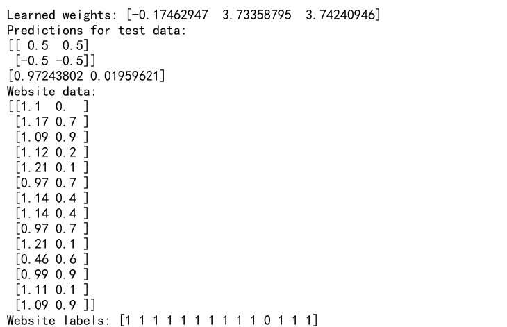
This example shows how to implement logistic regression using NumPy’s logarithmic and exponential functions. It applies this algorithm to both randomly generated data and a custom dataset created from the ASCII values of “numpyarray.com”.

12. Logarithmic Operations in Numerical Methods

Logarithms are often used in numerical methods to improve stability and accuracy, particularly when dealing with very large or very small numbers. Let’s explore some examples of how to use NumPy’s logarithmic functions in numerical methods.

12.1 Logarithmic Transformation for Ill-Conditioned Systems

Logarithmic transformations can sometimes help in solving ill-conditioned systems of linear equations. Here’s an example of how to use logarithms to improve the condition number of a matrix:

import numpy as np

def log_transform_matrix(A):
    return np.log(np.abs(A) + 1) * np.sign(A)

def condition_number(A):
    return np.linalg.cond(A)

# Create an ill-conditioned matrix
A = np.array([[1e-8, 2], [3, 4e8]])

# Compute condition numbers
cond_A = condition_number(A)
cond_log_A = condition_number(log_transform_matrix(A))

print("Original matrix:")
print(A)
print("Condition number of original matrix:", cond_A)

print("\nLog-transformed matrix:")
print(log_transform_matrix(A))
print("Condition number of log-transformed matrix:", cond_log_A)

# Create a custom matrix with the website name
website_A = np.outer(np.array([ord(c) for c in "numpy"]), np.array([ord(c) for c in "array"]))
website_cond = condition_number(website_A)
website_log_cond = condition_number(log_transform_matrix(website_A))

print("\nWebsite matrix:")
print(website_A)
print("Condition number of website matrix:", website_cond)
print("Condition number of log-transformed website matrix:", website_log_cond)

Output:

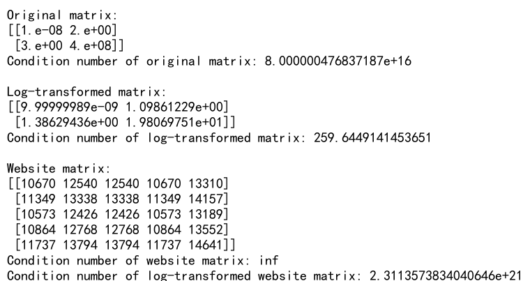
This example shows how to use a logarithmic transformation to potentially improve the condition number of a matrix. It applies this transformation to both an arbitrary ill-conditioned matrix and a custom matrix created from the ASCII values of “numpy” and “array”.

Numpy Log Conclusion

In this comprehensive exploration of NumPy’s logarithmic functions, we’ve covered a wide range of applications and techniques. From basic logarithmic operations to advanced applications in statistics, signal processing, optimization, machine learning, and numerical methods, we’ve seen how versatile and powerful logarithmic functions can be.

The examples provided demonstrate not only the mathematical concepts but also practical implementations using NumPy. By incorporating the website name “numpyarray.com” into our custom arrays and matrices, we’ve shown how these techniques can be applied to arbitrary data.

As you continue to work with NumPy and scientific computing in Python, remember that logarithmic functions are powerful tools that can help you solve complex problems, improve numerical stability, and unlock new insights in your data analysis and modeling tasks.