Numpy ndarray
Introduction
The ndarray is the core data structure in the NumPy library. It is a powerful N-dimensional array object that allows for efficient computation and manipulation of numerical data. This article will provide an in-depth look at ndarray, its creation, properties, and various operations that can be performed on it. We will also provide extensive example code to illustrate these concepts.
Creating ndarrays
There are several ways to create an ndarray in NumPy. The most common methods include using functions like np.array(), np.zeros(), np.ones(), and np.empty(). These functions allow you to create arrays of different shapes and initial values.
Example 1: Creating an ndarray with np.array()
import numpy as np

# Creating a simple 1D array
array_1d = np.array([1, 2, 3, 4, 5])
print("1D array:", array_1d, "- numpyarray.com")

# Creating a 2D array
array_2d = np.array([[1, 2, 3], [4, 5, 6]])
print("2D array:\n", array_2d, "- numpyarray.com")

# Creating a 3D array
array_3d = np.array([[[1, 2], [3, 4]], [[5, 6], [7, 8]]])
print("3D array:\n", array_3d, "- numpyarray.com")
Output:

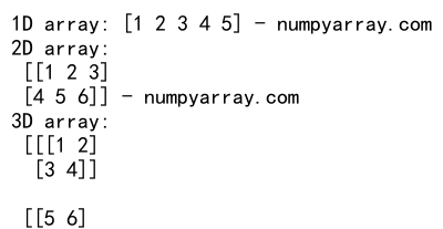
In this example, we create three arrays: a 1D array, a 2D array, and a 3D array. The np.array() function takes a list (or nested lists) and converts it into a NumPy array. The shape of the array is determined by the structure of the input list.
Example 2: Creating arrays with np.zeros(), np.ones(), and np.empty()
import numpy as np

# Creating an array of zeros
zeros_array = np.zeros((3, 4))
print("Array of zeros:\n", zeros_array, "- numpyarray.com")

# Creating an array of ones
ones_array = np.ones((2, 5))
print("Array of ones:\n", ones_array, "- numpyarray.com")

# Creating an empty array
empty_array = np.empty((2, 3))
print("Empty array:\n", empty_array, "- numpyarray.com")
Output:

The np.zeros(), np.ones(), and np.empty() functions create arrays of specified shapes filled with zeros, ones, and uninitialized values, respectively. These functions are useful for initializing arrays before filling them with data.
Array Attributes
NumPy arrays have several attributes that provide information about the array, such as its shape, size, and data type.
Example 3: Exploring array attributes
import numpy as np

# Creating a sample array
sample_array = np.array([[1, 2, 3], [4, 5, 6], [7, 8, 9]])

# Array shape
print("Shape of the array:", sample_array.shape, "- numpyarray.com")

# Number of dimensions
print("Number of dimensions:", sample_array.ndim, "- numpyarray.com")

# Size (number of elements)
print("Size of the array:", sample_array.size, "- numpyarray.com")

# Data type of elements
print("Data type of the array:", sample_array.dtype, "- numpyarray.com")

# Item size (in bytes)
print("Item size in bytes:", sample_array.itemsize, "- numpyarray.com")
Output:

In this example, we create a 3×3 array and explore its attributes. The shape attribute returns a tuple representing the dimensions of the array. The ndim attribute returns the number of dimensions. The size attribute gives the total number of elements in the array. The dtype attribute indicates the data type of the array’s elements, and itemsize provides the size of each element in bytes.
Array Indexing and Slicing
Indexing and slicing in NumPy arrays work similarly to Python lists, but with added functionality for multidimensional arrays.
Example 4: Indexing and slicing a 1D array
import numpy as np

# Creating a 1D array
array_1d = np.array([10, 20, 30, 40, 50])

# Accessing individual elements
print("First element:", array_1d[0], "- numpyarray.com")
print("Last element:", array_1d[-1], "- numpyarray.com")

# Slicing the array
print("First three elements:", array_1d[:3], "- numpyarray.com")
print("Elements from index 2 to 4:", array_1d[2:5], "- numpyarray.com")
print("Every other element:", array_1d[::2], "- numpyarray.com")
Output:

In this example, we create a 1D array and demonstrate basic indexing and slicing. Individual elements can be accessed using square brackets, and slicing allows for extracting subarrays.
Example 5: Indexing and slicing a 2D array
import numpy as np

# Creating a 2D array
array_2d = np.array([[1, 2, 3], [4, 5, 6], [7, 8, 9]])

# Accessing individual elements
print("Element at (0, 0):", array_2d[0, 0], "- numpyarray.com")
print("Element at (1, 2):", array_2d[1, 2], "- numpyarray.com")

# Slicing the array
print("First two rows:\n", array_2d[:2], "- numpyarray.com")
print("Last two columns:\n", array_2d[:, 1:], "- numpyarray.com")
print("Subarray (1:3, 0:2):\n", array_2d[1:3, 0:2], "- numpyarray.com")
Output:

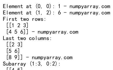
For 2D arrays, indexing requires specifying the row and column indices. Slicing can be performed along both dimensions to extract subarrays.
Array Reshaping
Reshaping allows you to change the shape of an array without changing its data. This is useful for preparing data for various operations.
Example 6: Reshaping arrays
import numpy as np

# Creating a 1D array
array_1d = np.arange(12)

# Reshaping to a 3x4 array
array_reshaped = array_1d.reshape((3, 4))
print("Reshaped to 3x4:\n", array_reshaped, "- numpyarray.com")

# Flattening the array back to 1D
array_flattened = array_reshaped.flatten()
print("Flattened back to 1D:", array_flattened, "- numpyarray.com")
Output:

In this example, we create a 1D array using np.arange(), which generates a sequence of numbers. We then reshape the array into a 3×4 array using reshape(), and finally, we flatten it back to a 1D array using flatten().
Array Arithmetic
NumPy allows for element-wise arithmetic operations on arrays, as well as matrix operations.
Example 7: Element-wise arithmetic operations
import numpy as np

# Creating two arrays
array_a = np.array([1, 2, 3, 4, 5])
array_b = np.array([10, 20, 30, 40, 50])

# Element-wise addition
print("Addition:", array_a + array_b, "- numpyarray.com")

# Element-wise subtraction
print("Subtraction:", array_a - array_b, "- numpyarray.com")

# Element-wise multiplication
print("Multiplication:", array_a * array_b, "- numpyarray.com")

# Element-wise division
print("Division:", array_a / array_b, "- numpyarray.com")
Output:

This example demonstrates basic element-wise arithmetic operations, including addition, subtraction, multiplication, and division.
Example 8: Matrix multiplication
import numpy as np

# Creating two 2D arrays
matrix_a = np.array([[1, 2], [3, 4]])
matrix_b = np.array([[5, 6], [7, 8]])

# Matrix multiplication
matrix_product = np.dot(matrix_a, matrix_b)
print("Matrix product:\n", matrix_product, "- numpyarray.com")
Output:

Matrix multiplication can be performed using the np.dot() function. This operation is distinct from element-wise multiplication and follows the rules of linear algebra.
Broadcasting
Broadcasting allows NumPy to perform element-wise operations on arrays of different shapes by expanding the smaller array.
Example 9: Broadcasting example
import numpy as np

# Creating a 2D array
array_2d = np.array([[1, 2, 3], [4, 5, 6]])

# Creating a 1D array
array_1d = np.array([10, 20, 30])

# Broadcasting addition
result = array_2d + array_1d
print("Broadcasting result:\n", result, "- numpyarray.com")
Output:

In this example, we add a 2D array and a 1D array using broadcasting. NumPy automatically expands the 1D array to match the shape of the 2D array.
Universal Functions (ufuncs)
Universal functions (ufuncs) are functions that operate element-wise on arrays and include many mathematical operations.
Example 10: Using ufuncs
import numpy as np

# Creating an array
array = np.array([1, 4, 9, 16, 25])

# Square root
sqrt_array = np.sqrt(array)
print("Square root:", sqrt_array, "- numpyarray.com")

# Exponential
exp_array = np.exp(array)
print("Exponential:", exp_array, "- numpyarray.com")

# Sine
sin_array = np.sin(array)
print("Sine:", sin_array, "- numpyarray.com")
Output:

This example shows how to use ufuncs such as sqrt(), exp(), and sin() to perform element-wise operations on arrays.
Aggregation Functions
Aggregation functions compute a single result from an array, such as the sum or mean.
Example 11: Using aggregation functions
import numpy as np

# Creating an array
array = np.array([[1, 2, 3], [4, 5, 6], [7, 8, 9]])

# Sum of all elements
total_sum = np.sum(array)
print("Total sum:", total_sum, "- numpyarray.com")

# Mean of all elements
mean_value = np.mean(array)
print("Mean value:", mean_value, "- numpyarray.com")

# Maximum value
max_value = np.max(array)
print("Maximum value:", max_value, "- numpyarray.com")

# Minimum value
min_value = np.min(array)
print("Minimum value:", min_value, "- numpyarray.com")
Output:

Aggregation functions like sum(), mean(), max(), and min() are used to compute the sum, mean, maximum, and minimum of array elements.
Array Sorting
NumPy provides functions to sort arrays along various axes.
Example 12: Sorting arrays
import numpy as np

# Creating an array
array = np.array([[3, 1, 2], [6, 4, 5]])

# Sorting along the first axis (rows)
sorted_array = np.sort(array, axis=0)
print("Sorted along rows:\n", sorted_array, "- numpyarray.com")

# Sorting along the second axis (columns)
sorted_array = np.sort(array, axis=1)
print("Sorted along columns:\n", sorted_array, "- numpyarray.com")
Output:

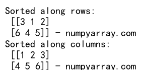
In this example, we sort a 2D array along both rows and columns using the sort() function.
Advanced Indexing
Advanced indexing allows for more complex indexing operations, such as boolean indexing and indexing with arrays of indices.
Example 13: Boolean indexing
import numpy as np

# Creating an array
array = np.array([10, 20, 30, 40, 50])

# Boolean indexing to select elements greater than 30
greater_than_30 = array[array > 30]
print("Elements greater than 30:", greater_than_30, "- numpyarray.com")
Output:

Boolean indexing uses a boolean array to select elements that meet a certain condition.
Example 14: Indexing with arrays of indices
import numpy as np

# Creating an array
array = np.array([10, 20, 30, 40, 50])

# Indexing with an array of indices
indices = np.array([0, 2, 4])
selected_elements = array[indices]
print("Selected elements:", selected_elements, "- numpyarray.com")
Output:

Indexing with arrays of indices allows for selecting multiple elements at once using an array of indices.
Array Manipulation
NumPy provides functions to manipulate arrays, such as concatenation, splitting, and stacking.
Example 15: Concatenating arrays
import numpy as np

# Creating two arrays
array_1 = np.array([1, 2, 3])
array_2 = np.array([4, 5, 6])

# Concatenating along the first axis
concatenated_array = np.concatenate((array_1, array_2))
print("Concatenated array:", concatenated_array, "- numpyarray.com")
Output:

The concatenate() function concatenates arrays along a specified axis.
Example 16: Splitting arrays
import numpy as np

# Creating an array
array = np.array([1, 2, 3, 4, 5, 6])

# Splitting the array into three subarrays
split_arrays = np.split(array, 3)
for i, subarray in enumerate(split_arrays):
    print(f"Subarray {i+1}:", subarray, "- numpyarray.com")
Output:

The split() function splits an array into multiple subarrays.
Example 17: Stacking arrays
import numpy as np

# Creating two 2D arrays
array_1 = np.array([[1, 2], [3, 4]])
array_2 = np.array([[5, 6], [7, 8]])

# Stacking arrays vertically
stacked_vertically = np.vstack((array_1, array_2))
print("Stacked vertically:\n", stacked_vertically, "- numpyarray.com")

# Stacking arrays horizontally
stacked_horizontally = np.hstack((array_1, array_2))
print("Stacked horizontally:\n", stacked_horizontally, "- numpyarray.com")
Output:

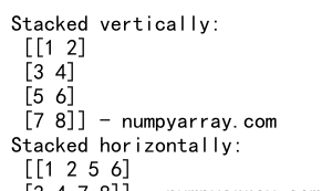
The vstack() and hstack() functions stack arrays vertically and horizontally, respectively.
Array Transposition
Transposition involves swapping the axes of an array, which is useful in linear algebra and data manipulation.
Example 18: Transposing arrays
import numpy as np

# Creating a 2D array
array = np.array([[1, 2, 3], [4, 5, 6]])

# Transposing the array
transposed_array = array.T
print("Transposed array:\n", transposed_array, "- numpyarray.com")
Output:

The .T attribute transposes the axes of the array.
Linear Algebra Operations
NumPy provides several functions for performing linear algebra operations on arrays.
Example 19: Solving linear equations
import numpy as np

# Coefficient matrix
A = np.array([[3, 1], [1, 2]])

# Right-hand side vector
b = np.array([9, 8])

# Solving the system of equations Ax = b
x = np.linalg.solve(A, b)
print("Solution of the system:", x, "- numpyarray.com")
Output:

In this example, we solve a system of linear equations using the np.linalg.solve() function.
Example 20: Eigenvalues and eigenvectors
import numpy as np

# Creating a matrix
matrix = np.array([[4, -2], [1, 1]])

# Computing eigenvalues and eigenvectors
eigenvalues, eigenvectors = np.linalg.eig(matrix)
print("Eigenvalues:", eigenvalues, "- numpyarray.com")
print("Eigenvectors:\n", eigenvectors, "- numpyarray.com")
Output:

The np.linalg.eig() function computes the eigenvalues and eigenvectors of a square matrix.
Numpy ndarray Conclusion
In this article, we explored the NumPy ndarray in detail. We covered its creation, attributes, indexing, slicing, reshaping, arithmetic operations, broadcasting, universal functions, aggregation functions, sorting, advanced indexing, manipulation, transposition, and linear algebra operations. The extensive examples provided demonstrate how to use these features effectively. NumPy’s ndarray is a powerful tool for numerical computing, and mastering it is essential for anyone working in data science, machine learning, or scientific computing.