Mastering NumPy Random Normal Distribution: A Comprehensive Guide

Mastering NumPy Random Normal Distribution: A Comprehensive Guide

NumPy random normal distribution is a powerful tool for generating random numbers following a Gaussian (normal) distribution. This article will explore the various aspects of numpy random normal distribution, its applications, and how to use it effectively in your data analysis and scientific computing projects.

Introduction to NumPy Random Normal Distribution

NumPy random normal distribution is a fundamental concept in statistics and data science. It allows us to generate random numbers that follow a normal distribution, also known as a Gaussian distribution. This distribution is characterized by its bell-shaped curve and is widely used in various fields, including physics, biology, finance, and machine learning.

The numpy random normal function is part of the NumPy library, which is a powerful tool for numerical computing in Python. It provides an efficient way to generate random numbers following a normal distribution with specified parameters.

Let’s start with a simple example to demonstrate how to use numpy random normal:

import numpy as np

# Generate 5 random numbers from a normal distribution with mean 0 and standard deviation 1
random_numbers = np.random.normal(loc=0, scale=1, size=5)
print("Random numbers from numpyarray.com:", random_numbers)

Output:

In this example, we import NumPy and use the np.random.normal() function to generate 5 random numbers from a normal distribution with a mean (loc) of 0 and a standard deviation (scale) of 1. The size parameter specifies the number of random numbers to generate.

Understanding the Parameters of NumPy Random Normal

The numpy random normal function takes three main parameters:

1. loc: The mean (average) of the distribution.
2. scale: The standard deviation of the distribution.
3. size: The shape of the output array.

Let’s explore each of these parameters in more detail:

The ‘loc’ Parameter

The loc parameter represents the mean of the normal distribution. It determines the center of the bell curve. By default, it is set to 0, but you can change it to any value depending on your requirements.

Here’s an example of generating random numbers with a different mean:

import numpy as np

# Generate 10 random numbers from a normal distribution with mean 5 and standard deviation 1
random_numbers = np.random.normal(loc=5, scale=1, size=10)
print("Random numbers from numpyarray.com with mean 5:", random_numbers)

Output:

In this example, we set the loc parameter to 5, which shifts the center of the distribution to 5.

The ‘scale’ Parameter

The scale parameter represents the standard deviation of the normal distribution. It determines the spread of the distribution. A larger standard deviation results in a wider bell curve, while a smaller standard deviation produces a narrower curve.

Let’s see an example with a different standard deviation:

import numpy as np

# Generate 10 random numbers from a normal distribution with mean 0 and standard deviation 2
random_numbers = np.random.normal(loc=0, scale=2, size=10)
print("Random numbers from numpyarray.com with standard deviation 2:", random_numbers)

Output:

In this example, we set the scale parameter to 2, which increases the spread of the generated random numbers.

The ‘size’ Parameter

The size parameter determines the shape of the output array. It can be an integer or a tuple of integers. If it’s an integer, the function returns a 1D array with that many elements. If it’s a tuple, it returns an array with the specified shape.

Here’s an example of generating a 2D array of random numbers:

import numpy as np

# Generate a 3x3 array of random numbers from a normal distribution
random_array = np.random.normal(loc=0, scale=1, size=(3, 3))
print("2D array of random numbers from numpyarray.com:")
print(random_array)

Output:

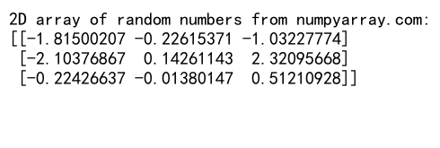
In this example, we use size=(3, 3) to generate a 3×3 array of random numbers.

Applications of NumPy Random Normal Distribution

NumPy random normal distribution has numerous applications in various fields. Let’s explore some of the common use cases:

Simulating Natural Phenomena

Many natural phenomena follow a normal distribution. For example, heights of individuals in a population, measurement errors, or thermal noise in electronic circuits. We can use numpy random normal to simulate these phenomena.

Here’s an example of simulating heights of individuals:

import numpy as np

# Simulate heights of 1000 individuals (in cm) with mean 170 and standard deviation 10
heights = np.random.normal(loc=170, scale=10, size=1000)
print("Simulated heights from numpyarray.com:", heights[:10])  # Print first 10 heights

Output:

This code generates 1000 random heights with a mean of 170 cm and a standard deviation of 10 cm.

Generating Noise in Machine Learning

In machine learning, adding random noise to data can help prevent overfitting and improve model generalization. NumPy random normal is often used for this purpose.

Here’s an example of adding noise to a simple dataset:

import numpy as np

# Create a simple dataset
X = np.linspace(0, 10, 100)
y = 2 * X + 1

# Add random noise to y
noise = np.random.normal(loc=0, scale=0.5, size=100)
y_noisy = y + noise

print("Original y from numpyarray.com:", y[:5])
print("Noisy y from numpyarray.com:", y_noisy[:5])

Output:

In this example, we create a simple linear dataset and add random noise to it using numpy random normal.

Monte Carlo Simulations

Monte Carlo simulations often use normal distributions to model uncertain variables. NumPy random normal is a valuable tool for such simulations.

Here’s a simple example of a Monte Carlo simulation to estimate the value of pi:

import numpy as np

def estimate_pi(n_points):
    x = np.random.normal(loc=0, scale=1, size=n_points)
    y = np.random.normal(loc=0, scale=1, size=n_points)
    inside_circle = np.sum(x**2 + y**2 <= 1)
    pi_estimate = 4 * inside_circle / n_points
    return pi_estimate

# Estimate pi using 100000 points
pi_estimate = estimate_pi(100000)
print("Estimated value of pi from numpyarray.com:", pi_estimate)

Output:

This code uses numpy random normal to generate random points and estimates the value of pi based on the ratio of points falling inside a unit circle.

Advanced Techniques with NumPy Random Normal

Now that we’ve covered the basics, let’s explore some advanced techniques using numpy random normal.

Generating Correlated Random Variables

Sometimes, we need to generate random variables that are correlated with each other. We can use numpy random normal along with the Cholesky decomposition to achieve this.

Here’s an example of generating two correlated random variables:

import numpy as np

# Define the correlation matrix
correlation_matrix = np.array([[1, 0.5], [0.5, 1]])

# Generate correlated random variables
n_samples = 1000
L = np.linalg.cholesky(correlation_matrix)
uncorrelated = np.random.normal(size=(2, n_samples))
correlated = np.dot(L, uncorrelated)

print("Correlated random variables from numpyarray.com:")
print(correlated[:, :5])  # Print first 5 pairs

Output:

This code generates two sets of random variables with a correlation coefficient of 0.5.

Generating Random Numbers with Constraints

Sometimes, we need to generate random numbers that satisfy certain constraints. We can use numpy random normal in combination with other NumPy functions to achieve this.

Here’s an example of generating positive random numbers:

import numpy as np

# Generate 1000 positive random numbers
positive_numbers = np.abs(np.random.normal(loc=0, scale=1, size=1000))
print("Positive random numbers from numpyarray.com:", positive_numbers[:10])

Output:

In this example, we use the np.abs() function to ensure all generated numbers are positive.

Generating Random Numbers from a Truncated Normal Distribution

A truncated normal distribution is a normal distribution with specified lower and upper bounds. While NumPy doesn’t have a built-in function for this, we can create one using numpy random normal and rejection sampling.

Here’s an example:

import numpy as np

def truncated_normal(mean, std, lower, upper, size):
    samples = np.random.normal(mean, std, size=size)
    while np.any((samples < lower) | (samples > upper)):
        invalid = (samples < lower) | (samples > upper)
        n_invalid = np.sum(invalid)
        samples[invalid] = np.random.normal(mean, std, size=n_invalid)
    return samples

# Generate 1000 random numbers from a truncated normal distribution
truncated_samples = truncated_normal(mean=0, std=1, lower=-2, upper=2, size=1000)
print("Truncated normal samples from numpyarray.com:", truncated_samples[:10])

Output:

This function generates random numbers from a normal distribution and rejects any values outside the specified bounds, replacing them with new samples until all values are within the bounds.

Visualizing NumPy Random Normal Distributions

Visualization is a powerful tool for understanding the properties of random distributions. Let’s explore how to visualize numpy random normal distributions using matplotlib.

Histogram of Random Normal Distribution

A histogram is a great way to visualize the shape of a normal distribution. Here’s how to create a histogram of random numbers generated using numpy random normal:

import numpy as np
import matplotlib.pyplot as plt

# Generate 10000 random numbers
random_numbers = np.random.normal(loc=0, scale=1, size=10000)

# Create a histogram
plt.hist(random_numbers, bins=50, density=True)
plt.title("Histogram of Random Normal Distribution from numpyarray.com")
plt.xlabel("Value")
plt.ylabel("Frequency")
plt.show()

Output:

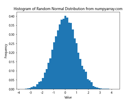
This code generates 10000 random numbers and creates a histogram to visualize their distribution.

Q-Q Plot for Normality Check

A Q-Q (Quantile-Quantile) plot is used to check if a dataset follows a normal distribution. Here’s how to create a Q-Q plot using numpy random normal:

import numpy as np
import matplotlib.pyplot as plt
import scipy.stats as stats

# Generate 1000 random numbers
random_numbers = np.random.normal(loc=0, scale=1, size=1000)

# Create Q-Q plot
fig, ax = plt.subplots()
stats.probplot(random_numbers, dist="norm", plot=ax)
ax.set_title("Q-Q Plot of Random Normal Distribution from numpyarray.com")
plt.show()

Output:

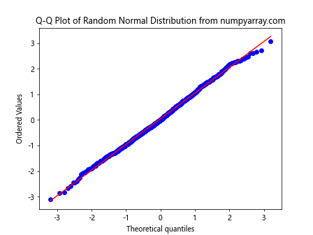
This code generates 1000 random numbers and creates a Q-Q plot to check if they follow a normal distribution.

Comparing NumPy Random Normal with Other Distributions

While the normal distribution is widely used, it’s important to understand how it compares to other distributions. Let’s compare numpy random normal with some other common distributions.

Normal vs Uniform Distribution

The uniform distribution generates random numbers with equal probability across a specified range. Let’s compare it with the normal distribution:

import numpy as np
import matplotlib.pyplot as plt

# Generate random numbers
normal_numbers = np.random.normal(loc=0, scale=1, size=10000)
uniform_numbers = np.random.uniform(low=-3, high=3, size=10000)

# Create histograms
plt.hist(normal_numbers, bins=50, alpha=0.5, label="Normal")
plt.hist(uniform_numbers, bins=50, alpha=0.5, label="Uniform")
plt.title("Normal vs Uniform Distribution from numpyarray.com")
plt.xlabel("Value")
plt.ylabel("Frequency")
plt.legend()
plt.show()

Output:

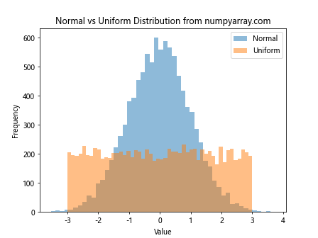
This code generates random numbers from both normal and uniform distributions and plots their histograms for comparison.

Normal vs Exponential Distribution

The exponential distribution is often used to model the time between events in a Poisson process. Let’s compare it with the normal distribution:

import numpy as np
import matplotlib.pyplot as plt

# Generate random numbers
normal_numbers = np.random.normal(loc=1, scale=0.5, size=10000)
exponential_numbers = np.random.exponential(scale=1, size=10000)

# Create histograms
plt.hist(normal_numbers, bins=50, alpha=0.5, label="Normal")
plt.hist(exponential_numbers, bins=50, alpha=0.5, label="Exponential")
plt.title("Normal vs Exponential Distribution from numpyarray.com")
plt.xlabel("Value")
plt.ylabel("Frequency")
plt.legend()
plt.show()

Output:

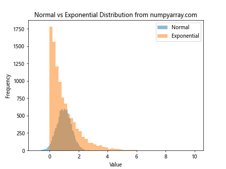
This code generates random numbers from both normal and exponential distributions and plots their histograms for comparison.

Statistical Analysis with NumPy Random Normal

NumPy random normal is not just useful for generating random numbers, but also for statistical analysis. Let’s explore some statistical techniques using numpy random normal.

Confidence Intervals

Confidence intervals are used to estimate the range of values that is likely to contain the true population parameter. Here’s how to calculate a confidence interval for the mean using numpy random normal:

import numpy as np
import scipy.stats as stats

# Generate a sample of 100 random numbers
sample = np.random.normal(loc=10, scale=2, size=100)

# Calculate the mean and standard error
sample_mean = np.mean(sample)
sample_std = np.std(sample, ddof=1)
standard_error = sample_std / np.sqrt(len(sample))

# Calculate 95% confidence interval
confidence_level = 0.95
degrees_freedom = len(sample) - 1
t_value = stats.t.ppf((1 + confidence_level) / 2, degrees_freedom)
margin_of_error = t_value * standard_error

confidence_interval = (sample_mean - margin_of_error, sample_mean + margin_of_error)

print("95% Confidence Interval from numpyarray.com:", confidence_interval)

Output:

This code generates a sample of random numbers, calculates the sample mean and standard error, and then computes a 95% confidence interval for the population mean.

Hypothesis Testing

Hypothesis testing is a fundamental technique in statistics. Let’s use numpy random normal to perform a one-sample t-test:

import numpy as np
from scipy import stats

# Generate a sample of 100 random numbers
sample = np.random.normal(loc=10, scale=2, size=100)

# Perform one-sample t-test
hypothesized_mean = 9.5
t_statistic, p_value = stats.ttest_1samp(sample, hypothesized_mean)

print("T-statistic from numpyarray.com:", t_statistic)
print("P-value from numpyarray.com:", p_value)

Output:

This code generates a sample of random numbers and performs a one-sample t-test to determine if the sample mean is significantly different from a hypothesized population mean.

Practical Applications of NumPy Random Normal in Data Science

NumPy random normal has numerous practical applications in data science. Let’s explore a few examples.

Bootstrapping

Bootstrapping is a resampling technique used to estimate the sampling distribution of a statistic. Here’s an example of using numpy random normal for bootstrapping:

import numpy as np

def bootstrap_mean(data, n_bootstrap=1000):
    bootstrap_means = np.zeros(n_bootstrap)
    for i in range(n_bootstrap):
        bootstrap_sample = np.random.choice(data, size=len(data), replace=True)
        bootstrap_means[i] = np.mean(bootstrap_sample)
    return bootstrap_means

# Generate a sample dataset
data = np.random.normal(loc=10, scale=2, size=100)

# Perform bootstrapping
bootstrap_means = bootstrap_mean(data)

# Calculate confidence interval
confidence_interval = np.percentile(bootstrap_means, [2.5, 97.5])

print("95% Bootstrap Confidence Interval from numpyarray.com:", confidence_interval)

Output:

This code generates a sample dataset, performs bootstrapping to estimate the sampling distribution of the mean, and calculates a 95% confidence interval.

Feature Engineering

In machine learning, feature engineering often involves adding noise or creating synthetic features. NumPy random normal can be useful for these tasks. Here’s an example of adding noise to create a new feature:

import numpy as np

# Create a sample dataset
X = np.random.uniform(0, 10, size=(100, 2))

# Add a noisy feature
noise = np.random.normal(loc=0, scale=0.5, size=100)
X_with_noise = np.column_stack((X, X[:, 0] + noise))

print("Dataset with noisy feature from numpyarray.com:")
print(X_with_noise[:5])

Output:

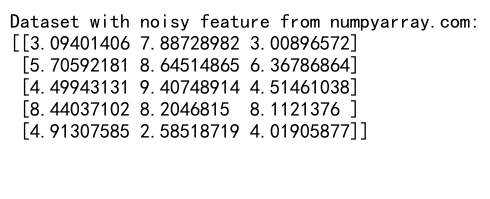
This code creates a sample dataset and adds a new feature that is a noisy version of an existing feature.

Anomaly Detection

Anomaly detection often involves identifying data points that deviate significantly from the normal distribution. Here’s a simple example using numpy random normal:

import numpy as np

def detect_anomalies(data, threshold=3):
    mean = np.mean(data)
    std = np.std(data)
    z_scores = np.abs((data - mean) / std)
    return z_scores > threshold

# Generate normal data with some anomalies
normal_data = np.random.normal(loc=0, scale=1, size=1000)
anomalies = np.random.normal(loc=5, scale=1, size=20)
data = np.concatenate([normal_data, anomalies])

# Detect anomalies
is_anomaly = detect_anomalies(data)

print("Number of anomalies detected from numpyarray.com:", np.sum(is_anomaly))

Output:

This code generates a dataset with mostly normal data and some anomalies, then uses a simple z-score method to detect the anomalies.

Best Practices for Using NumPy Random Normal

When working with numpy random normal, there are several best practices to keep in mind:

1. Seed the random number generator: For reproducibility, it’s important to set a seed for the random number generator. This ensures that you get the same sequence of random numbers each time you run your code.

import numpy as np

np.random.seed(42)  # Set a seed for reproducibility
random_numbers = np.random.normal(loc=0, scale=1, size=5)
print("Random numbers from numpyarray.com:", random_numbers)

Output:

2. Use appropriate parameters: Make sure to use appropriate values for the loc and scale parameters based on your specific use case.

3. Consider the size of your output: Be mindful of the size parameter, especially when generating large arrays of random numbers, as it can impact memory usage.

4. Vectorize operations: When possible, use vectorized operations instead of loops to improve performance.

5. Check for normality: If you’re assuming normality in your analysis, it’s a good practice to check if your data actually follows a normal distribution.

Common Pitfalls and How to Avoid Them

When working with numpy random normal, there are some common pitfalls to be aware of:

1. Forgetting to set a seed: This can lead to irreproducible results. Always set a seed when you need reproducibility.

2. Misunderstanding parameters: Make sure you understand what the loc and scale parameters represent (mean and standard deviation, respectively).

3. Generating inappropriate sample sizes: Be cautious about generating very large samples, as they can consume a lot of memory.

4. Assuming normality without checking: Always verify if your data actually follows a normal distribution before applying techniques that assume normality.

5. Misinterpreting results: Remember that random numbers, even from a normal distribution, can sometimes produce unexpected patterns. Don’t over-interpret random fluctuations.

NumPy random normal distribution Conclusion

NumPy random normal is a powerful tool for generating random numbers from a normal distribution. It has wide-ranging applications in statistics, data science, machine learning, and many other fields. By understanding how to use numpy random normal effectively, you can simulate complex phenomena, add controlled noise to your data, perform statistical analyses, and much more.

Remember to always consider the specific requirements of your project when using numpy random normal. Pay attention to the parameters you’re using, ensure reproducibility by setting seeds when necessary, and always validate your assumptions about the distribution of your data.